Ah I see why the plots were misleading…
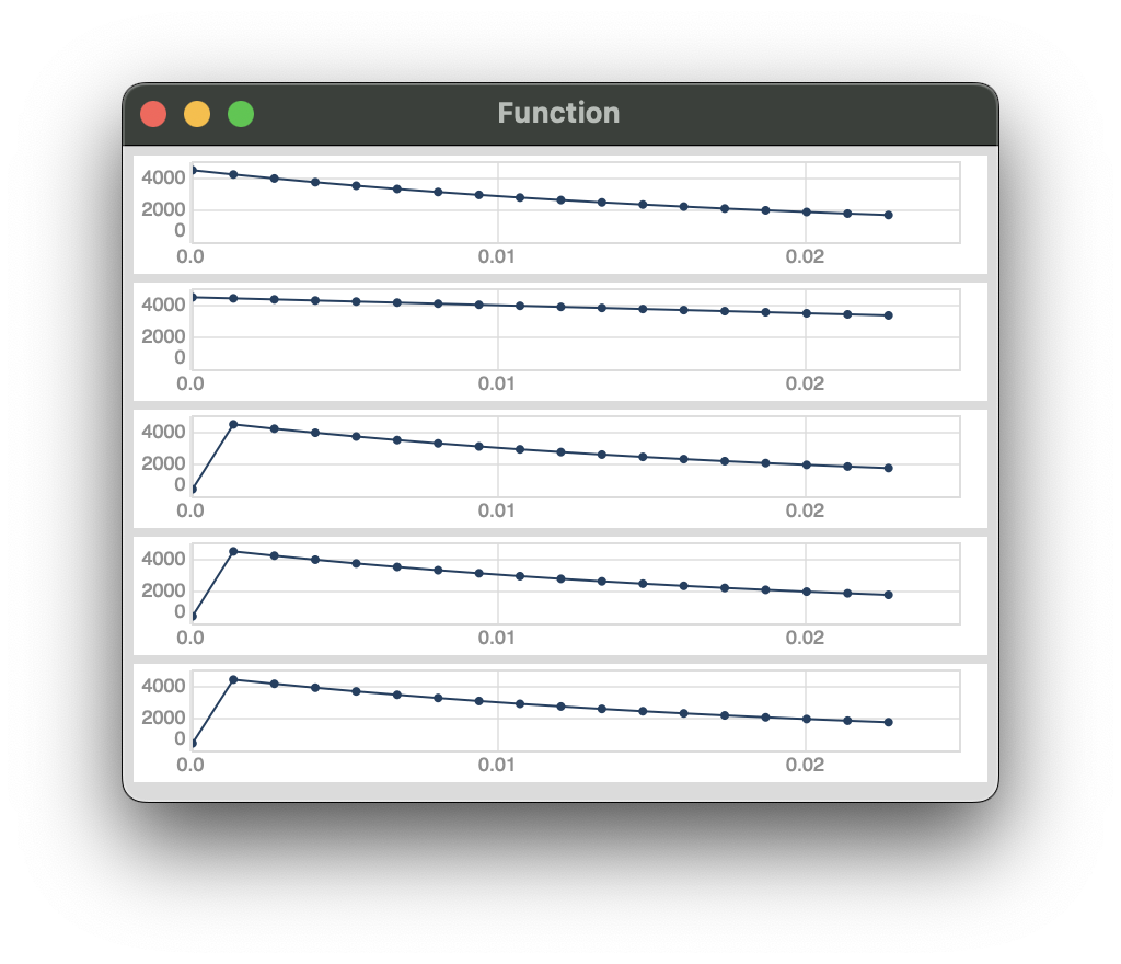
Plotting only the frequency envelopes show the correct behavior (IMO), i.e. an “immediate” (but still non-zero) onset from perc’s initial level of 0.
(
p = {
	var egs = [
		EnvGen.kr(Env([1, 0], 0.08, curve: -4)), // -4 is the default \perc curve
		EnvGen.kr(Env([1, 0], [0.081])),
		EnvGen.kr(Env.perc(0, 0.08)),
		EnvGen.kr(Env.perc(0.001, 0.08)),
		// even A2K on an ar envelope doesn't fix this!
		A2K.kr(EnvGen.ar(Env.perc(0.001, 0.08))),
	];
	var modFactor = 8;
	var freq = 500;
	var freqs = freq * (1 + (modFactor * egs));
	var sig = RLPF.ar(Saw.ar(100), freqs, 0.3);
	// [freqs, sig].lace(egs.size*2)
	freqs
}.plot(0.025).plotMode_(\dlines);

// { p.specs = [[0, 5000], [-1, 1]].dup(p.value.size).flatten(1) }.defer(1)
)
There is no repeated sample, but because you were plotting both k-rate and a-rate signals together, it upsamples the k-rate signals using K2A, which imposes a 1-block lag on the values.
This wouldn’t be an issue if we follow through with this idea of giving K2A a transition time argument.