Related to this thread about filtering behavior –
Here’s one of my classroom demos that explains a bit more about what is happening with filters. This is one of my favorite topics – I get kinda excited about it  so it’s a bit long post. Work through the examples one by one.
To start with, let’s do something seemingly trivial: take a signal, and output the average between successive samples.
s.boot;

b = Buffer.read(s, Platform.resourceDir +/+ "sounds/a11wlk01.wav");

// original sample
(
a = {
	var sig = PlayBuf.ar(1, b, loop: 0, doneAction: 2);
	sig.dup
}.play;
)

// two-point averaging filter
(
a = {
	var sig = PlayBuf.ar(1, b, loop: 0, doneAction: 2);
	var previous = Delay1.ar(sig);
	((sig + previous) * 0.5).dup
}.play;
)
It’s hard to hear, but in fact, high frequencies are attenuated. (This is LPZ1 in SC.)
A filter’s impulse response is what you get when feeding a single 1.0 sample into the filter:
// averaging filter, fed an impulse (graph)
(
a = {
	var sig = Impulse.ar(0);
	var previous = Delay1.ar(sig);
	[sig, (sig + previous) * 0.5]
}.plot(duration: 32/44100);
)
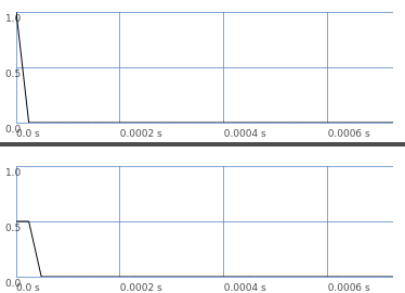
In this graph, the left channel is nonzero for one sample, and then silent. The right channel (filter) is nonzero for two samples.
So: A filter’s output is always longer than the input. You can’t do filtering without extending the duration.
Instead of an average, you could take the difference between successive samples. This is a rather severe high pass filter (HPZ1).
// two-point difference filter
(
a = {
	var sig = PlayBuf.ar(1, b, loop: 0, doneAction: 2);
	var previous = Delay1.ar(sig);
	((sig - previous) * 0.5).dup
}.play;
)

// difference filter, impulse response (graph)
(
a = {
	var sig = Impulse.ar(0);
	var previous = Delay1.ar(sig);
	[sig, (sig - previous) * 0.5]
}.plot(duration: 32/44100);
)

These filters can be expressed as:
// averaging filter
this output sample = (0.5 * current input sample) + (0.5 * previous input sample)

// difference filter
this output sample = (0.5 * current input sample) + (-0.5 * previous input sample)

OR:

y(i) = 0.5 * x(i) + 0.5 * x(i-1)  // avg
y(i) = 0.5 * x(i) + -0.5 * x(i-1)  // diff
So the averaging filter has coefficients a0 = 0.5 and a1 = 0.5, while the difference filter has coefficients a0 = 0.5 and a1 = -0.5. These are feedforward coefficients.
Now look at the impulse response graphs. The average filter’s IR is 0.5, 0.5, 0… and the difference filter’s IR is 0.5, -0.5, 0… exactly matching the coefficients.
In fact, it continues like this. You can have an impulse response of any length, and use those samples as feedforward coefficients: y(i) = sum[over k = 0..n-1](IR(k) * x(i-k)). This is convolution.
The impulse response has a finite length – so, convolution against a finite impulse response is the same as a finite-impulse-response filter (FIR).
// make an IR for the difference filter
k = Buffer.alloc(s, 2048, 1);

k.zero;
k.setn(0, [0.5, -0.5]);

(
a = {
	var sig = PlayBuf.ar(1, b, loop: 0);
	var filt = Convolution2.ar(sig, k, framesize: k.numFrames);
	DetectSilence.ar(filt, doneAction: 2);
	filt.dup
}.play;
)
So we put the impulse response into a buffer and use fixed-frame convolution on the signal, and… it sounds like the difference filter.
We can do the same with a more interesting filter.
(
{
	var sig = Impulse.ar(0);
	var filt = RLPF.ar(sig, 2000, 0.05);
	// HERE: Save the impulse response into 'k'
	RecordBuf.ar(filt, k, loop: 0);
	[sig, filt]
}.plot(duration: k.numFrames / s.sampleRate);
)
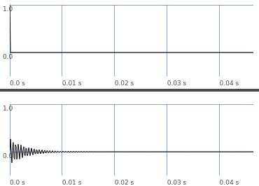
This is a nice sinusoidal decay. Technically, it never reaches exactly 0 – so this is an infinite impulse response (IIR). Practically, it eventually gets close enough to zero that we don’t have to record it forever.
You get an IIR by feeding the filter’s output samples back into the filter – so then you have both feedforward and feedback coefficients. y(i) = (a0 * x(i)) + (a1 * x(i-1)) + (a2 * x(i-2)) + (b1 * y(i-1)) + (b2 * y(i-2)) is a second-order filter because it goes back two samples. This formula is also called biquad and it’s the basis of most of SC’s standard filters.
A second-order filter tapers off by 12 dB/oct. A third-order filter goes back three samples and tapers off by 18 dB/oct; fourth-order, four samples, 24 dB/oct. Because of limitations in floating point precision, usually fourth-order filters are implemented as a chain of two equivalent second-order filters: RLPF.ar(RLPF.ar(sig, freq, rq), freq, rq).
OK, compare convolution against the filter UGen:
// convolution against filter's impulse response
(
a = {
	var sig = PlayBuf.ar(1, b);
	var filt = Convolution2.ar(sig, k, framesize: k.numFrames);
	DetectSilence.ar(filt, doneAction: 2);
	filt.dup
}.play;
)

// compare to RLPF
(
a = {
	var sig = PlayBuf.ar(1, b);
	var filt = RLPF.ar(sig, 2000, 0.05);
	DetectSilence.ar(filt, doneAction: 2);
	filt.dup
}.play;
)
And… they sound the same.
So what is the filter’s frequency response?
The impulse response is the time domain response. FFT converts this to frequency domain.
// get frequency response
k.getToFloatArray(wait: -1, action: { |data| d = data.postln });

f = d.as(Signal).fft(Signal.newClear(d.size), Signal.fftCosTable(d.size));

// 'fft' result consists of complex numbers (Cartesian coordinates)
// but we want magnitudes (the lengths of the polar vectors)
f = f.asPolar;

// FFT is a mirror image around the center
// so use only the first half
f.rho[0 .. d.size div: 2].plot;
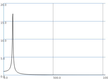
… which plots 1.0 amplitude for the lowest frequencies, leading up to a resonant “hump,” and tapering off to zero at the highest frequencies – as you would expect for a low pass filter with resonance. (It looks biased to the left because the frequency axis is linear here. Frequency scopes usually convert to a logarithmic scale. The peak frequency is f.rho[0 .. d.size div: 2].maxIndex * (s.sampleRate / k.numFrames) = 2002.587, given an input frequency of 2000  )
)
hjh