There are some ugens which have a band-limited and non-band-limited versions in SC. For instance the Pulse ugen generate band-limited signal, whereas LFPulse creats non-band-limited pulses. What is the difference between band-limited and non-limited ugens? At least to my ear both Pulse and LFPulse sound exactly the same.
So, the reason this is hearable in the higher frequencies, is that LFPulse passes through also other frequencies near the center frequency?
No.
What you’re hearing is aliasing, an unavoidable mathematical fact of digital audio. There should be many pages online about it – it’s a fundamental concept.
hjh
Thanks, to my understanding aliasing is about relation between sampling frequency and the signal, how could it be related to the filters and filter bands? That confuses me!
Try this: foldover
1 Like
There’s a temptation to think that aliasing can be filtered away. That is only possible in very special cases. It’s like a spice in a meal that you cannot simply remove after you have added it – you might like the flavour though ![]()
2 Likes
This might help you understand - it is in Pd but it explains in the most musician-friendly why harmonics will fold at Nyquist.

2 Likes
Interesting to plot them - shows some clear differences:
{[LFPulse.ar(400), Pulse.ar(400)]}.plot(0.01, bounds: 800 @ 500, minval: -1, maxval: 1);
{[LFSaw.ar(400), Saw.ar(400)]}.plot(0.01, bounds: 800 @ 500, minval: -1, maxval: 1);
There is a miscalculation in the example here, right? The foldover signal should be 11 Khz?
This is indeed interesting! The band-limited signals seem to have an amplitude in the range -0.5, 0.5
Do you know why is this the case?
for example if one tries to generate a 13,000 Hz. signal when the sampling rate is 11,000 HZ then the signal will be folded over to 9,000 HZ. (11,000 - 2,000)
Indeed @amt, this is incorrect.
Corrected: “for example if one tries to generate a 13,000 Hz. signal when the Nyquist frequency is 11,000 HZ (sampling rate = 22000 Hz) then the signal will be folded over to 9,000 HZ. (11,000 - 2,000 – also, 22000 - 13000 = 9000)”
hjh
1 Like
Very interesting (and subtle) point.
A pulse waveform that is exactly balanced, e.g. n samples up, n samples down, has no aliasing.
s.boot;

b = { LFPulse.ar(SampleRate.ir / 16, mul: 2, add: -1) }.getToFloatArray(1024 / s.sampleRate, action: { |data| d = data.postln });

// this pure square wave doesn't need a window
// but the next one will need it
// So let's keep things apples-to-apples

d = d * Signal.hanningWindow(d.size);
d.plot

// FFT
f = d.as(Signal).fft(Signal.newClear(d.size), Signal.fftCosTable(d.size));
f = f.asPolar;

f.rho[0 .. d.size div: 2].plot;
… and you’ll see four harmonics. This is as expected, according to the Nyquist theorem: frequency = sample rate / 16 = Nyquist / 8, so in theory you could see harmonics 1 to 8. But a square wave includes only odd harmonics, so you see 1, 3, 5 and 7.
The plot uses a linear frequency scale, so it isn’t clear that it’s a high frequency – but it is. Find the index of that first peak, and then scale it up to the sample rate:
i = f.rho.detectIndex(_ > 200);  // 63

i * s.sampleRate / 1024  // at 48kHz, 2953.125
… which is very close to the input frequency. (The Hann window must be affecting the pitch slightly.)
If the frequency is not an integer factor of the sample rate, then the up-vs-down cycles can’t be balanced.
b = { LFPulse.ar(SampleRate.ir / 16.2, mul: 2, add: -1) }.getToFloatArray(1024 / s.sampleRate, action: { |data| d = data.postln });

// 8s with occasional 9s
d.as(Array).separate(_ != _).collect(_.size)
Most of the blocks of consecutive equivalent values are 8 samples long, but sometimes one is 9 samples.
In order to stretch/push/squeeze the samples into that irregular shape, the spectrum must contain extra frequencies… and we see them. Repeat the FFT part:
d = d * Signal.hanningWindow(d.size);
d.plot

f = d.as(Signal).fft(Signal.newClear(d.size), Signal.fftCosTable(d.size));

f = f.asPolar;

f.rho[0 .. d.size div: 2].plot
… and you see a LOT of junk.
So aliasing is related to the asymmetry in the unbalanced waveform.
When the frequency is very high, the push/pull is a relatively large percentage of the wavelength – so the alias frequencies must be strong enough to hear. At lower frequencies, it’s a much smaller percentage, and accordingly, the amount of energy in aliased frequencies is significantly less (maybe inaudible).
hjh
3 Likes
I’m not sure why. I tried forcing the range to (-1,1), but it doesn’t seem to make a difference to the range seen on the plot:
{[LFPulse.ar(391), Pulse.ar(391).range(-1, 1)]}.plot(0.01, bounds: 800 @ 500, minval: -1, maxval: 1);
{[LFSaw.ar(391), Saw.ar(391).range(-1, 1)]}.plot(0.01, bounds: 800 @ 500, minval: -1, maxval: 1);
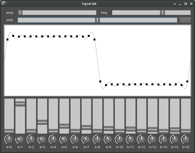
I have an interesting graphical demonstration of that: A few years ago, I hacked up a GUI that oversamples a 32-point signal. If you put a geometrically perfect 32-sample square wave into it:
// run the big block, then:

// square = 16x +0.7, 16x -0.7
e.data = Array.fill(z div: 2, [0.7, -0.7]).lace(z);
… it looks like a true bandlimited square, complete with Gibbs effect, in between the samples.

But… pull the FFT out of that, and normalize it against its maximum magnitude, and:
e.fft.rho / e.fft.rho.maxItem

-> [ 0.0, 1.0, 0.0, 0.33765868917828, 0.0, 0.20792919291452, 0.0, 0.15450533035176, 0.0, 0.12679923770497, 0.0, 0.11114046832904, 0.0, 0.10242762415687, 0.0, 0.09849141074536, 0.0, 0.09849141074536, 0.0, 0.10242765224407, 0.0, 0.11114046686992, 0.0, 0.12679924945131, 0.0, 0.15450531860542, 0.0, 0.2079291879641, 0.0, 0.33765864269487, 0.0, 0.99999992864426 ]
… in fact, there is some excess energy. The third partial should be 1/3, but is 0.33766 (about 0.004 too high); the fifth partial should be 1/5, but is 0.20793 (0.008 too high).
I hadn’t noticed this before.
In the GUI, you can also “correct” the FFT and display it:
p = e.fft.deepCopy;
m = p.rho.maxItem;

p.rho.do { |mag, i| p.rho[i] = if(mag < 0.001) { 0.0 } { m / max(i, 1) } };

e.fft = p;
… and then the samples go just a little bit wiggly.
A common trick for synthesizing a pulse wave is to subtract a delayed copy of a sawtooth. When the pulse width is 0.5, this will leave about half the amplitude.
(
{
	var freq = 391, pulseWidth = 0.5;
	var saw = Saw.ar(freq);
	[
		LFPulse.ar(freq),
		Pulse.ar(freq, pulseWidth),
		saw - DelayC.ar(saw, 1, pulseWidth / freq)
	]
}.plot(0.01, bounds: 800 @ 500, minval: -1, maxval: 1);
)
Here, the amplitudes are about the same between the Pulse vs saw - DelayC (although Pulse seems to take more time for DC to stabilize).
hjh
Let SC do it for you automatically!
(Please correct me if the arithmetic below is wrong!)
(
{
	var freq, sr, in, freqFollowed, hasFreq;
	sr = SampleRate.ir;
	in = SoundIn.ar(0);
	# freqFollowed, hasFreq = Pitch.kr(in, minFreq: 16, maxFreq: sr / 2);
	freq = MouseY.kr(440, sr);
	[freq, freqFollowed, sr - freq].poll;
	SinOsc.ar(freq) * 0.01;
}.play
)
I am not sure about the information in the video: he says if playing a 23050 Hz tone on a machine with 44100 Hz sr, what we hear are two tones: one at 23050 Hz and the other at 21050 Hz?
This one doesn’t exist at all. It’s already folded over. It’s gone.
A sampled function cannot represent any frequency higher than half the sample rate, period, no exception. This is a 100% inescapable mathematical reality. At 44100 Hz, there is no 23000-anything Hz.
hjh
Try this:
(
{
	var simulatedSampleRates = [22050, 16000, 8000, 4000, 2000, 1000];
	var sinFreq = 1000;
	Latch.ar(SinOsc.ar(sinFreq), Impulse.ar(simulatedSampleRates))
}.plot
)
The farther down the window you go, the lower the simulated sample rate is. When you get to a sample rate that’s the same frequency as the signal, it just gives you one value because all of the movement of the sine wave is happening between the time that it’s being sampled. Like if you stand up when someone is facing away from you and then sit down before they turn back around.
It’ll also cause you to end up with frequencies that weren’t intended:
(
{
	var simulatedSampleRates = [22050, 4000, 2000, 2500];
	var sinFreq = 1000;
	Latch.ar(SinOsc.ar(sinFreq), Impulse.ar(simulatedSampleRates))
}.plot
)
The last plot looks like it only oscillates 5 cycles over the length of the plot instead of 10 as it should because of downsampling.
1 Like
This is a bit of a misleading point.
This result looks like it has a lower periodicity, but it is the digital representation of the 1000 Hz sine wave at 2500 Hz sampling rate (analogous to a 17640 Hz sine wave at 44.1 kHz).
The Nyquist frequency at 2500 Hz is 1250 Hz. 1000 is less than this, so there is no aliasing and no loss of this frequency information. If you up-sample the given (admittedly bizarre-looking) series of samples, you will get the 1000 Hz sine wave back, cleanly.
We can do that in SC.
(
p = {
	var simulatedSampleRates = [22050, 4000, 2000, 2500];
	var sinFreq = 1000;
	Latch.ar(SinOsc.ar(sinFreq), Impulse.ar(simulatedSampleRates))
}.plot
)

a = p.value.last;
a.size  // 480 since I'm at 48000 Hz now

// eliminate the zero-order hold
// this will give us the samples directly
a = a.separate { |a, b| a != b }.collect { |clump| clump[0] };

// a.size  // 25

// for FFT, we need a power of 2
a = a.wrapExtend(32);

// Because this does not wrap around exactly,
// we should apply a window
a = a * Signal.hanningWindow(a.size);
a.plot;

// At this point, the plot looks very messy

// Get the 32-point FFT = 16 distinct bins
// DC, bin 1, bin 2, 3, 4 ... 16 (this is Nyquist), 15, 14, 13, ... 2, 1
// = 32 bins, 16 distinct partials + DC
f = a.as(Signal).fft(Signal.newClear(a.size), Signal.fftCosTable(a.size)).asPolar;

// To up-sample, we need to manufacture more FFT bins
// The original bins are still 0 to 16 -- bandlimited!
// 17 etc. will all be zero energy
(
~insertZeros = { |array, newSize|
	var half = array.size div: 2;
	array[.. half]
	++
	Array.fill(newSize - array.size, 0)
	++
	array[half + 1 ..]
};

g = Polar(
	~insertZeros.(f.rho, 512),
	~insertZeros.(f.theta, 512)
);
)

// inverse FFT
g = g.asComplex;
h = g.real.as(Signal).ifft(g.imag.as(Signal), Signal.fftCosTable(g.real.size));

h.real.plot;  // show and tell
At this point, the magnitude is very small because of FFT normalization (the energy that had been spread over 32 samples is now spread out over 512) – but what you don’t see is a distorted sine wave (it’s clean) or a reduced frequency. (If it were true that the 2500 Hz plot reflected five cycles in the frame, then the IFFT here would show 6 or 7 cycles… but it doesn’t.)
There’s a brilliant video from xiph – the creators of the ogg format – where they take analog signal generators, oscilloscopes and frequency analyzers, and digitize the signal up to 20000 Hz @ 44.1 kHz (i.e. 2.205 samples per sine cycle!) and show that the DAC reconstruction to analog is still a pure sine wave. I think this video should be required viewing for all digital audio professionals – it efficiently disabuses the viewer of several misconceptions, about this, and dithering, and time resolution.
hjh
3 Likes