hey,
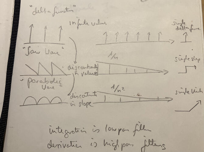
I would like to open this thread with a sketch, which i have drawn while watching one of the awesome classes by miller puckete and reading his book about two years ago (unfortunately cant remember which one it was, better watch them all).
We could take away from that sketch that lowpass filtering is integration while highpass filtering is derivation.
motivation
The whole reason i have investigated this topic FM vs. PM, is that im mostly using an approach, where i derive triggers and slopes from a scheduling phasor and run an accumulator based on Duty.ar(SampleDur.ir, trig, Dseries(0, 1)) which is been reset by the derived trigger, not to 0 but to the sub-sample offset for sub-sample accuracy. In this thread im explaining how you can derive sub-sample accurate events from phasor based scheduling.
The main problem is then the following:
One problem i have encountered lately when using these accumulators multiplied by a slope to scale your ramp signal wrapped between 0 and 1, is that you cant use FM on these.
The reason for that is a subtle difference between a continous ramp implementation based on
f(t) = m * x(t), where x(t) is our sample counter and m is our constant slope and f(t) = f(t-1) + m, where f(t-1) is our previous accumulated value stored in history and m is our constant slope.
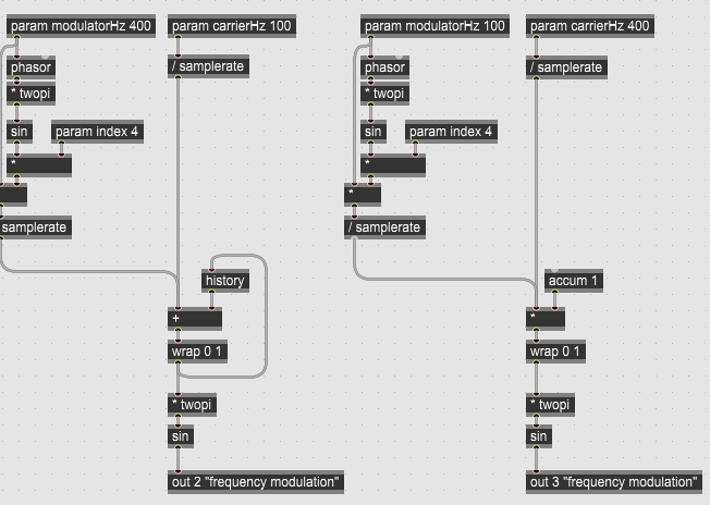
Let me show this in ~gen:
On the right side you have a continuous ramp signal (a phasor) which is based on a sample counter (accum 1), multiplied by a slope and wrapped between 0 and 1, where on the left side you have a continuous ramp signal, which is based on the combination of +, history and wrap between 0 and 1.
So without modulation f(t) = m * x(t), where x(t) is our sample counter and m is our constant slope is identical to f(t) = f(t-1) + m, where f(t-1) is our previous accumulated value stored in history and m is our constant slope. In the first case we are scaling a linear counter, while in the second we are integrating a varying increment over time.
If we adjust the formula for the accumulator to: f(t) = (m + b(t))* x(t), where b(t) is a time varying modulation compared to f(t) = f(t-1) + (m * b(t)) the result is not the same, because we are not integrating the time dependend modulation correctly.
So using (slope * accum).wrap(0, 1) instead of (history + slope).wrap(0, 1) is an edge case, which only behaves identical when the slope is latched for every single cycle of the accumulated phasor, and is therefore constant during one cycle.
So the general solution in low level DSP is to use switch, +, history for accumulating a continuous ramp signal (switch for the possibility of a reset, when receiving a trigger), which is capapable of FM.
But if we use (slope * accum).wrap(0, 1), which is the only option available in SC in this context, we can still do PM.
PM vs. FM
So lets start with implementing Phase Modulation (PM) vs. Frequency Modulation (FM).
Alot about this has already been said in this thread.
To produce exactly the same results with PM vs. FM, you just have to integrate your modulator.
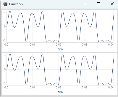
If your modulator is a sine wave thats easy:
Here using SinOsc as a modulator and SinOsc as a carrier signal for FM and PM:
(
{
	var carrFreq, modFreq, index;
	var pmod, fmod, pm, fm;

	carrFreq = 100;
	modFreq = 150;
	index = 2;

	pmod = 1 - (SinOsc.ar(modFreq, 0.5pi)) * index;
	pm = SinOsc.ar(carrFreq, pmod);

	fmod = SinOsc.ar(modFreq) * index;
	fm = SinOsc.ar(carrFreq + (modFreq * fmod));

	[pm, fm];

}.plot(0.041);
)
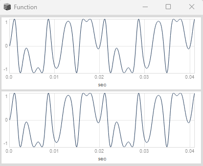
The same can be written if you drive your sin or cos functions with a Phasor (or if you think of driving your single-cycle waveforms stored in a buffer with a combination of BufRd and Phasor), it produces an identical result for FM and PM:
(
{
	var carrFreq, modFreq, index;
	var modPhase, pmod, fmod;
	var carrPhasePM, sigPM;
	var carrFreqFM, carrPhaseFM, sigFM;

	carrFreq = 100;
	modFreq = 150;
	index = 2;

	modPhase = Phasor.ar(DC.ar(0), modFreq * SampleDur.ir);

	pmod = 1 - cos(modPhase * 2pi) * 0.5 / pi * index;
	fmod = sin(modPhase * 2pi) * index;

	// PM
	carrPhasePM = Phasor.ar(DC.ar(0), carrFreq * SampleDur.ir);
	carrPhasePM = (carrPhasePM + pmod).wrap(0, 1);
	sigPM = sin(carrPhasePM * 2pi);

	// FM
	carrFreqFM = carrFreq + (modFreq * fmod);
	carrPhaseFM = Phasor.ar(DC.ar(0), carrFreqFM * SampleDur.ir);
	sigFM = sin(carrPhaseFM * 2pi);

	[sigPM, sigFM];

}.plot(0.041);
)
OnePole filters and PM vs. FM
But you dont have to integrate your modulator for PM explicitly.
You can use an abitrary modulator for PM when you plug it into a lowpass filter and use that same modulator for FM, which you plug into a highpass filter, where both are tuned to the same modulational frequency and they produce the same result.
Because lowpass filtering is integration while highpass filtering is derivation.
(
{
	var carrFreq, modFreq, index;
	var pmod, fmod, pm, fm;

	carrFreq = 100;
	modFreq = 150;
	index = 2;

	pmod = SinOsc.ar(modFreq) * index;
	pmod = OnePole.ar(pmod, exp(-2pi * modFreq * SampleDur.ir));
	pm = SinOsc.ar(carrFreq, pmod);

	fmod = SinOsc.ar(modFreq) * index;
	fmod = fmod - OnePole.ar(fmod, exp(-2pi * modFreq * SampleDur.ir));
	fm = SinOsc.ar(carrFreq + (modFreq * fmod));

	[pm, fm];

}.plot(0.041);
)
You could additionally multiply your filter frequency based on modFreq with a filterRatio param to get different kinds of flavours out of PM and FM.
If you multiply your modulator with the index before you apply the filter, this effect will be even more pronounced.
Using a OnePole filter is identical to using Lag, but with the difference that the filter coefficients, when implemented with the formula i have shown in the examples above are calculated based on frequency in Hz and not time in milliseconds.
I have made a really interesting discovery:
If you take an index window driven by the same modPhase as your PM modulator based on 1 - cos(modPhase * 2pi) * 0.5 / pi (1 - cos(modPhase * 2pi) * 0.5 is basically a hanning window, so both the index window and the PM modulator share the same phase) and compare it with FM, where your FM modulator is based on sin(modPhase * 2pi) multiplied by the same index window (the index window and the FM modulator dont share the same phase) PM and FM produce different results!
But if you take an index window driven by the same modPhase as your PM modulator based on sin(modPhase * 2pi) (the index window and the PM modulator dont share the same phase) an put it into a lowpass filter and compare it with FM, where your FM modulator is based on sin(modPhase * 2pi) multiplied by the same index window (the index window and the FM modulator also dont share the same phase) and put it into a highpass filter the result for PM and FM is identical!
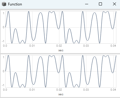
Lets see this on some plots:
// highpass filtering of FM and lowpass filtering of PM without index window (identical!!!)

(
{
	var carrFreq, modFreq, modPhase;
	var pmod, fmod;
	var carrPhasePM, carrFreqFM, carrPhaseFM;
	var index;
	var pm, fm;

	carrFreq = 100;
	modFreq = 400;

	modPhase = Phasor.ar(DC.ar(0), modFreq * SampleDur.ir);
	index = \index.kr(2);

	// PM
	pmod = sin(modPhase * 2pi) / 2pi * index;
	pmod = OnePole.ar(pmod, exp(-2pi * modFreq * SampleDur.ir));

	carrPhasePM = Phasor.ar(DC.ar(0), carrFreq * SampleDur.ir);
	carrPhasePM = (carrPhasePM + pmod).wrap(0, 1);
	pm = sin(carrPhasePM * 2pi);

	// FM
	fmod = sin(modPhase * 2pi) * index;
	fmod = fmod - OnePole.ar(fmod, exp(-2pi * modFreq * SampleDur.ir));

	carrFreqFM = carrFreq + (modFreq * fmod);
	carrPhaseFM = Phasor.ar(DC.ar(0), carrFreqFM * SampleDur.ir);
	fm = sin(carrPhaseFM * 2pi);

	[pm, fm];

}.plot(0.02);
)

// highpass filtering of FM and lowpass filtering of PM with index window (identical!!!)

(
{
	var carrFreq, modFreq, modPhase;
	var pmod, fmod;
	var carrPhasePM, carrFreqFM, carrPhaseFM;
	var indexWindow, index;
	var pm, fm;

	carrFreq = 100;
	modFreq = 400;

	modPhase = Phasor.ar(DC.ar(0), modFreq * SampleDur.ir);
	indexWindow = IEnvGen.ar(Env([0, 1, 0], [0.5, 0.5], \lin), modPhase);
	index = \index.kr(4) * indexWindow;

	// PM
	pmod = sin(modPhase * 2pi) / 2pi * index;
	pmod = OnePole.ar(pmod, exp(-2pi * modFreq * SampleDur.ir));

	carrPhasePM = Phasor.ar(DC.ar(0), carrFreq * SampleDur.ir);
	carrPhasePM = (carrPhasePM + pmod).wrap(0, 1);
	pm = sin(carrPhasePM * 2pi);

	// FM
	fmod = sin(modPhase * 2pi) * index;
	fmod = fmod - OnePole.ar(fmod, exp(-2pi * modFreq * SampleDur.ir));

	carrFreqFM = carrFreq + (modFreq * fmod);
	carrPhaseFM = Phasor.ar(DC.ar(0), carrFreqFM * SampleDur.ir);
	fm = sin(carrPhaseFM * 2pi);

	[pm, fm];

}.plot(0.02);
)


// integration of PM modulator to match FM without index window (identical!!!)

(
{
	var carrFreq, modFreq, modPhase;
	var pmod, fmod;
	var carrPhasePM, carrFreqFM, carrPhaseFM;
	var index;
	var pm, fm;

	carrFreq = 100;
	modFreq = 400;

	modPhase = Phasor.ar(DC.ar(0), modFreq * SampleDur.ir);
	index = \index.kr(2);

	// PM
	pmod = 1 - cos(modPhase * 2pi) * 0.5 / pi * index;
	carrPhasePM = Phasor.ar(DC.ar(0), carrFreq * SampleDur.ir);
	carrPhasePM = (carrPhasePM + pmod).wrap(0, 1);
	pm = sin(carrPhasePM * 2pi);

	// FM
	fmod = sin(modPhase * 2pi) * index;
	carrFreqFM = carrFreq + (modFreq * fmod);
	carrPhaseFM = Phasor.ar(DC.ar(0), carrFreqFM * SampleDur.ir);
	fm = sin(carrPhaseFM * 2pi);

	[pm, fm];

}.plot(0.02);
)

// integration of PM modulator to match FM with index window (not identical!!!!)

(
{
	var carrFreq, modFreq, modPhase;
	var pmod, fmod;
	var carrPhasePM, carrFreqFM, carrPhaseFM;
	var indexWindow, index;
	var pm, fm;

	carrFreq = 100;
	modFreq = 400;

	modPhase = Phasor.ar(DC.ar(0), modFreq * SampleDur.ir);
	indexWindow = IEnvGen.ar(Env([0, 1, 0], [0.5, 0.5], \lin), modPhase);
	index = \index.kr(2) * indexWindow;

	// PM
	pmod = 1 - cos(modPhase * 2pi) * 0.5 / pi * index;
	carrPhasePM = Phasor.ar(DC.ar(0), carrFreq * SampleDur.ir);
	carrPhasePM = (carrPhasePM + pmod).wrap(0, 1);
	pm = sin(carrPhasePM * 2pi);

	// FM
	fmod = sin(modPhase * 2pi) * index;
	carrFreqFM = carrFreq + (modFreq * fmod);
	carrPhaseFM = Phasor.ar(DC.ar(0), carrFreqFM * SampleDur.ir);
	fm = sin(carrPhaseFM * 2pi);

	[pm, fm];

}.plot(0.02);
)
Without further ado the modulational index of PM and FM, when FM is implemented with carrFreq + (modFreq * fmod * index) and the PM modulator is scaled correctly by dividing by number of cycles in radians is identical.
One interesting discovery here is that the formula for the PM modulator to get the same index like in FM with sin(modPhase * 2pi) is 1 - cos(modPhase * 2pi) * 0.5 / pi where 1 - cos(modPhase * 2pi) * 0.5 is actually a hanning window divided by pi, with half a cycle vs. sin(modPhase * 2pi) / 2pi with one full cycle into a lowpass filter.
Multiplying by 0.5 and then dividing by pi is the same as dividing by 2pi, but the main take away here is that the division is based on the number of cycles of the modulator in radians to match PM and FM.
This becomes maybe clearer if we dont implement FM with carrFreq + (modFreq * fmod * index), where the modulational index is dependent on the frequency of the modulator, where a higher modulational frequency leads to a higher modulational index and vice versa.
I often times implement FM like this carrFreq + (carrFreq * fmod * index), where the modulational index for FM insnt based on the modulators frequency but on the carrier frequency.
The reason for that is, that otherwise low frequency modulators lead to small indices of modulation. But i found out that i can create the sounds im mostly interested in with low modulational frequencies and high indices.
If you want to implement PM where the modulational index is scaled by the carrFreq instead of the modFreq you have to multiply your modulator by the ratio of (carrFreq / modFreq).
(
{
	var carrFreq, modFreq, index;
	var modPhase, pmod, fmod;
	var carrPhasePM, sigPM;
	var carrFreqFM, carrPhaseFM, sigFM;

	carrFreq = 100;
	modFreq = 50;
	index = 3;

	modPhase = Phasor.ar(DC.ar(0), modFreq * SampleDur.ir);

	pmod = 1 - cos(modPhase * 2pi) * 0.5 / pi * index * (carrFreq / modFreq);
	fmod = sin(modPhase * 2pi) * index;

	// PM
	carrPhasePM = Phasor.ar(DC.ar(0), carrFreq * SampleDur.ir);
	carrPhasePM = (carrPhasePM + pmod).wrap(0, 1);
	sigPM = sin(carrPhasePM * 2pi);

	// FM
	carrFreqFM = carrFreq + (carrFreq * fmod);
	carrPhaseFM = Phasor.ar(DC.ar(0), carrFreqFM * SampleDur.ir);
	sigFM = sin(carrPhaseFM * 2pi);

	[sigPM, sigFM];

}.plot(0.02);
)
