How does SuperCollider Smoothen the sound? It sounds way too different than Pd and without clicks

[porres]

Forever I have noticed how SuperCollider sounds kinda different than Pure Data, but I seem to have finally nailed down an example that shows it quite clearly. Take this for instance.

// decay tone
({var env = Env([1, 0], [1]).ar;
(SinOsc.ar(440, pi/2) * env)!2}.play)

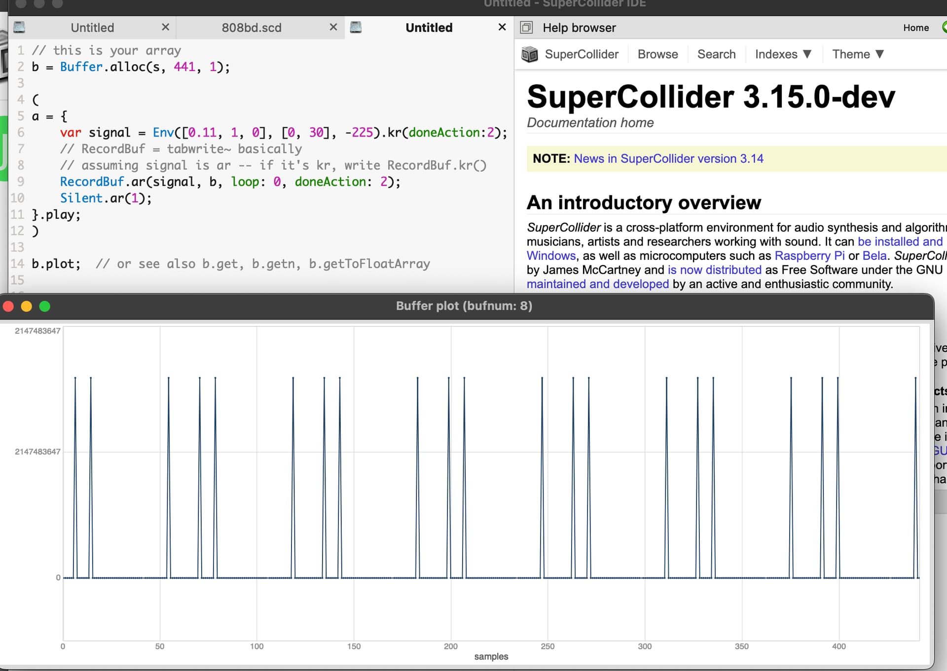
An equivalent Pd patch is:

Now, You can test SuperCollider yourselves, and I basically hear no click when jumping from o to 1!

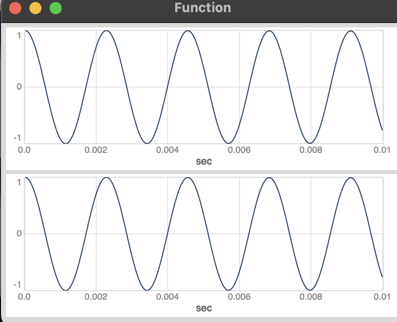
I can plot it with

(
{ var env = Env([1, 0], [1]).ar;
(SinOsc.ar(440, pi/2) * env)!2
}.plot(0.01);
)

and see this

But I can’t hear it…

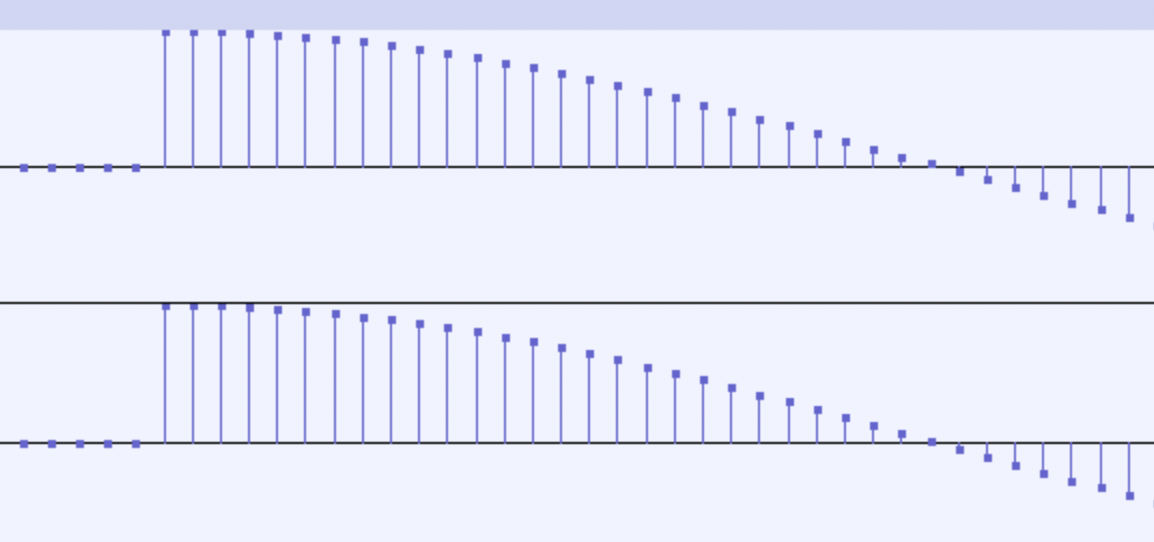
I have recorded the Pd patch output and here it is. Watch out, it’s loud…

There’s nothing wrong with the file and it sounds as I’d expect, with a harsh click, and it looks proper in Audacity and just like it’s plotted in Sc…

I have to say that if you have mechanisms to prevent clicks and stuff you’re interfering too much with the sound, and this makes it rather hard to port patches from one system to the other, if not impossible.

Anyway, please point me to all that makes SuperCollider probably sound different than other environments, such as PD and MAX (by the way, an equivalent MAX patch sounds exactly the same).

cheers
Alex

[porres]

for me, SC sounds like feeding “1 9, 0 991 9” to [vline~] in Pd, which means about 10ms smoothening

[josh]

Control rates are, in general, smoother (linear interpolations) in SC UGen code

/*
Josh Parmenter
www.realizedsound.net/josh
*/

[bsssssss]

Yes this is because the play method has a fadeTime parameter which default to 0.02, so to make your example work as expected you can do:

// decay tone
({var env = Env([1, 0], [1]).ar;
(SinOsc.ar(440, pi/2) * env)!2}.play(fadeTime: 0))

Also making a synthdef instead and sending it to the server will not introduce fade times.
More info here and here.

[jamshark70]

@porres

I have to say that if you have mechanisms to prevent clicks and stuff you’re interfering too much with the sound…

bsssssss 's answer is correct: when you use a convenience method like Function:play, the convenience method might also add other conveniences, and you might not need every convenience in every case. The extra convenience here is a fade-in, fade-out trapezoidal envelope, which is absent from your Pd example.

An analogy in pd might be an abstraction that wraps another abstraction in an envelope. You use the enveloper abstraction and say “but there’s an envelope, that’s interfering with the sound” – and the solution is, don’t use the abstraction, just do the synthesis directly.

When convenience methods don’t handle the exact requirement, then the solution is to fall back to more fundamental components, in this case, SynthDef (which adds no additional envelope).

I use {}.play for prototyping, and for launching longer-running synths where the fade-in is over long before you’ll ever hear anything from the larger process. If I need precise envelope control, SynthDef it is, never {}.play.

hjh

[porres]

ok, it’s .play’s fault then, cool. What about other things I should be aware of?

@josh

Control rates are, in general, smoother (linear interpolations) in SC UGen code

I am aware of that, and that’s also making it way harder to port to Pd.

For instance, I am dealing with this kick drum

( // bass drum
{
var decay=30, amp=2, tone=50;
var fenv, env, trienv, sig, sub, punch, pfenv;

env = Env([0.11, 1, 0], [0, decay], -225).kr(doneAction:2);
trienv = Env([0.11, 0.6, 0], [0, decay], -230).kr;
fenv = Env([tone*7, tone*1.35, tone], [0.05, 0.6], -14).kr;
pfenv = Env([tone*7, tone*1.35, tone], [0.03, 0.6], -10).kr;

sig = SinOsc.ar(fenv, pi/2) * env;
sub = LFTri.ar(fenv, pi/2) * trienv * 0.05;
punch = HPF.ar(SinOsc.ar(pfenv, pi/2) * env * 2, 350);

(Limiter.ar((sig + sub + punch) * 2.5, 0.5) * amp)!2;

}.play(fadeTime: 0);
)

changing env, trienv, fenv and pfenv to “.ar” instead of “.kr” does change the quality a lot!

In ‘.kr’ it sounds way more mullfed/smoother…

[porres]

@porres

In ‘.kr’ it sounds way more mullfed/smoother…

So, how can I effectively render the samples of an envelope in ‘.kr’ and check the exact sample per sample output just to be sure and then compare to what I am generating in Pd?

For Pd it’s quite easy, I just use tabwrite~ and check the values on a table.

I’ve been struggling with this and there doesn’t seem to be a simple way to do this and inspect the values

[alikthename]

@porres

In ‘.kr’ it sounds way more mullfed/smoother…

kr is lower sampling rate, by default 1 sample for 64 audiorate samples.
if your patch in pd is all in audiorate (like 44100) use .ar
also for better overal accuracy just stick to ar everywhere in synthdefs

[alikthename]

@porres

For Pd it’s quite easy, I just use tabwrite~ and check the values on a table.

you can record to buffer and plot

you also can scope the server output (Server.local.scope)

but you already used audacity, I think it’s the most flexible if OS allows you to easily connect sc → audacity

[porres]

@alikthename

you can record to buffer and plot

I wouldn’t know the steps to do any of that, and plotting is not like having an array in Pd where you can check the values.

I wouldn’t know how to record a short snippet and open it in audacity like I did with Pd.

And I know Pd is like ‘.ar’, the problem is porting a code like I shared that is based on ‘.kr’ envelopes

[prko]

like this?

/* plotting a simple envelope-controlled cosine wave */

(
x = {
	var env = Env([1, 0], [0.1]).ar;
	(SinOsc.ar(440, pi/2) * env)!2
};
x.play(fadeTime:0);

x.plot(0.1); // change the window width!!!!

x.plotAudio(0.1) // change the window width!!!!
)


/* writing audio data to a buffer and using it in sequence */

(
s.waitForBoot { 
	var duration = 1;
	var numChannels = 2;
	~bufferTest = Buffer.alloc(s, s.sampleRate * duration, numChannels);
	
	SynthDef(\CosineWithEnv, { |out = 0, freq = 440, phase = (pi/2), dur = 1, bufnum = 0, rate = 1|
		var env = Env([1, 0], [dur]).ar(Done.freeSelf);
		var sig = SinOsc.ar(freq, phase) * env ! 2;
		var phasor = Phasor.ar(0, BufRateScale.kr(bufnum) * rate, 0, BufFrames.kr(bufnum));
		BufWr.ar(sig, bufnum, phasor);
		Out.ar(out, sig)
	}
	).add;
	
	s.sync;
	
	Synth(\CosineWithEnv, [bufnum: ~bufferTest, dur: duration]);
	
	duration.wait;
	
	~bufferTest.plot; // change the window width!!!!
	// ~bufferTest.play
}
)


/* writing audio data to a buffer step by step */

(
~dur = 0.1;
~bufferTest_ = Buffer.alloc(s, s.sampleRate * ~dur, 2);
)

Synth(\CosineWithEnv, [bufnum: ~bufferTest_, dur: ~dur])

~bufferTest_.plot // change the window width!!!!

~bufferTest_.play

[jamshark70]

@porres

For Pd it’s quite easy, I just use tabwrite~ and check the values on a table.

For SC it’s almost that easy.

// this is your array
b = Buffer.alloc(s, howManySamplesDoIWantToRecord, 1);

(
a = {
	var signal = theSignalIWantToRecord;
	// RecordBuf = tabwrite~ basically
	// assuming signal is ar -- if it's kr, write RecordBuf.kr()
	RecordBuf.ar(signal, b, loop: 0, doneAction: 2);
	Silent.ar(1);
}.play;
)

b.plot;  // or see also b.get, b.getn, b.getToFloatArray

Alternately,

p = { ... audio or kr stuff... }.plot;

p.value[channelIndex]  // this is an array of sample values

Most plot examples don’t assign it to a variable, but all the data are available through the plotter object.

@porres

So, how can I effectively render the samples of an envelope in ‘.kr’ and check the exact sample per sample output just to be sure and then compare to what I am generating in Pd?

Since Pd doesn’t have any concept of control rate, you don’t want to render the samples of an envelope at .kr and check against Pd’s audio rate envelope.

It would be relevant to look at the conversion of the control rate envelope up to audio rate: K2A.ar(krEnvelope).

What you will find, at that extreme curve value, is a series of line segments, each 64 samples long, quickly dropping to near zero (for the decay). This precise signal will be prohibitively difficult to generate in Pd. I think you’re wasting your time to try to replicate this curve exactly.

One weird thing is that you’ve specified a 30-second decay, but with a really kind of outrageous curve value. The decay segment reaches pretty close to 0 within one second. So why not just write a one-second decay with a more moderate curve? Then your volume envelope will be able to release the synth after one second instead of after 30 seconds.

An attack time of 0 is something I would never recommend to my students. 2 or 3 ms is fine for percussion.

I think if you clean up the envelope definition, the difference between ar and kr will be greatly reduced. Then you have less of a moving target to try to imitate in Pd.

The difference between ar and kr here is especially in the attack segment, where the curve (way too big a curve value IMO) causes it to rise extremely quickly. kr then effectively acts like a slew limiter. So it’s a bit convoluted: generating a near instantaneous rise, but at control rate so that it will be slowed down, and then trying to mirror this behavior in Pd. If you define the desired envelope shape in simpler terms (times matching the actual perceived rise/fall times, curves within +/- 5, there is usually not much need to have curves outside of this range), it will be simpler to port.

hjh

[porres]

@jamshark70

One weird thing is that you’ve specified a 30-second decay, but with a really kind of outrageous curve value. The decay segment reaches pretty close to 0 within one second. So why not just write a one-second decay with a more moderate curve? Then your volume envelope will be able to release the synth after one second instead of after 30 seconds.

This is not my patch, it is just a patch I am trying to port to Pd, and I have realized all that

here’s where I got it from. This is supposed to be a TR-808 BassDrum, but it’s part of a broader research of mine gathering many TR-808 approximations. By the way, the portedplugins has an analog bass drum, which is from Mutable Instruments, and I am also porting this code to a Pd external from the plaits module.

I would eventually rewrite this to a more sane code as I also think this 30 second long envelope is rather clumsy…

Nonetheless, I want to start by faithfully reproducing this original code result.

[porres]

@jamshark70

Since Pd doesn’t have any concept of control rate, you don’t want to render the samples of an envelope at .kr and check against Pd’s audio rate envelope.

But I can generate an audio with this envelope in .kr and then check on a buffer/table what it effectively results in.

I reckon the code is weird, but in order to simplify it, I need to understand what it is actually doing…

I believe that, for instance this part

Env([0.11, 1, 0], [0, decay], -225).kr

Goes immediatelly to 0.11, causing a moderate click, then it goes to 1 within a block size, rising in linear interpolation, and then it decays?

Anyway, I was just having trouble plotting and checking it. I will try the suggestions, but if it is easy to tell me what actually happens I’d be thankful.

cheers

[jamshark70]

@porres

Anyway, I was just having trouble plotting and checking it.

Actually I think .plot is the easiest way. This isn’t commonly mentioned, because usually we just {}.plot without assigning to a variable, so you can’t manipulate the plotter. But as I mentioned, p = {}.plot instead, and then you can use p.value to get a 2d array, where p.value[0] is an array of sample values for the first channel, p.value[1] is the array of samples for the second channel and so on. Then, you could re-plot portions of a channel etc.

@porres

believe that, for instance this part

Env([0.11, 1, 0], [0, decay], -225).kr

Goes immediatelly to 0.11, causing a moderate click, then it goes to 1 within a block size, rising in linear interpolation, and then it decays?

At kr it’s actually slightly weirder than that. It starts at 0.11 (again, which I’d never do – code posted online is not necessarily trustworthy), holds at 0.11 for one control block, then linearly rises to 1.0 in the duration of a control block. This “minimum duration” for a segment was implemented to fix some bug, which I forget. I’m not crazy about this behavior; I just remember it was done for some reason. But you can ignore what is basically a one block delay in the envelope triggering.

Then it decays, but not in a smooth curve. Rather the decay happens in 64-sample line segments.

The linear ramp when upsampling the kr values to ar is what I meant by slew limiting.

hjh

[prko]

@jamshark70

RecordBuf.ar(signal, b, loop: 0, doneAction: 2);

RecordBuf is better than BufWr. Sorry!

[porres]

Ok, yeah, that behaviour is not intuitive, and it definitely doesn’t seem elegant. It seems the code was just messed a lot with by ear until reaching a satisfactory result. I will try to design more intuitive and meaningful envelopes that sound about the same.

@jamshark70

Then it decays, but not in a smooth curve. Rather the decay happens in 64-sample line segments.

The linear ramp when upsampling the kr values to ar is what I meant by slew limiting.

what I understand is that .kr is like a sample and hold and collects sample values at block boundaries. But then, it gets linearly interpolated, right?

[porres]

@prko

like this?

not really, this only shows me the graph, nut not the values, and I just needed something simple to test how the .kr envelope renders, your code had more stuff

[porres]

@jamshark70

For SC it’s almost that easy

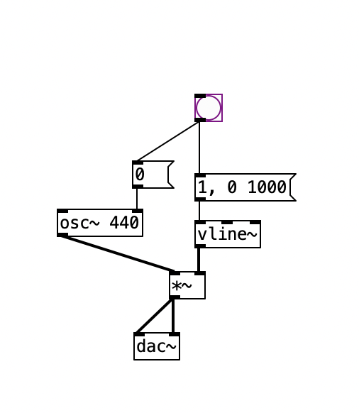
well, I tried this and the result didn’t seem right

the code

// this is your array
b = Buffer.alloc(s, 441, 1);

(
a = {
var signal = Env([0.11, 1, 0], [0, 30], -225).kr(doneAction:2);
// RecordBuf = tabwrite~ basically
// assuming signal is ar – if it’s kr, write RecordBuf.kr()
RecordBuf.ar(signal, b, loop: 0, doneAction: 2);
Silent.ar(1);
}.play;
)

b.plot;

[prko]

@porres

not really, this only shows me the graph, nut not the values, and I just needed something simple to test how the .kr envelope renders, your code had more stuff

Then, lke this?

(
{
	var env = Env([1, 0], [1]).ar(Done.freeSelf);
        // var env = Env([1, 0], [1]).kr(Done.freeSelf); 
	(SinOsc.ar(440, pi/2) * env.poll)!2
}.play(fadeTime: 0)
)

-> Synth('temp__38' : 1047)
UGen(EnvGen): 1
UGen(EnvGen): 0.9
UGen(EnvGen): 0.8
UGen(EnvGen): 0.7
UGen(EnvGen): 0.6
UGen(EnvGen): 0.5
UGen(EnvGen): 0.4
UGen(EnvGen): 0.3
UGen(EnvGen): 0.2
UGen(EnvGen): 0.1
UGen(EnvGen): 8.60799e-15

or:

(
{
	var env = Env([1, 0], [1]).ar(Done.freeSelf);
        // var env = Env([1, 0], [1]).kr(Done.freeSelf); 
	(SinOsc.ar(440, pi/2) * env.poll(40))!2
}.play(fadeTime: 0)
)

-> Synth('temp__39' : 1048)
UGen(EnvGen): 1
UGen(EnvGen): 0.975
UGen(EnvGen): 0.95
UGen(EnvGen): 0.925
UGen(EnvGen): 0.9
UGen(EnvGen): 0.875
UGen(EnvGen): 0.85
UGen(EnvGen): 0.825
UGen(EnvGen): 0.8
UGen(EnvGen): 0.775
UGen(EnvGen): 0.75
UGen(EnvGen): 0.725
UGen(EnvGen): 0.7
UGen(EnvGen): 0.675
UGen(EnvGen): 0.65
UGen(EnvGen): 0.625
UGen(EnvGen): 0.6
UGen(EnvGen): 0.575
UGen(EnvGen): 0.55
UGen(EnvGen): 0.525
UGen(EnvGen): 0.5
UGen(EnvGen): 0.475
UGen(EnvGen): 0.45
UGen(EnvGen): 0.425
UGen(EnvGen): 0.4
UGen(EnvGen): 0.375
UGen(EnvGen): 0.35
UGen(EnvGen): 0.325
UGen(EnvGen): 0.3
UGen(EnvGen): 0.275
UGen(EnvGen): 0.25
UGen(EnvGen): 0.225
UGen(EnvGen): 0.2
UGen(EnvGen): 0.175
UGen(EnvGen): 0.15
UGen(EnvGen): 0.125
UGen(EnvGen): 0.1
UGen(EnvGen): 0.075
UGen(EnvGen): 0.05
UGen(EnvGen): 0.025
UGen(EnvGen): 8.60799e-15