How to calculate phase synchrony?

[rodet]

hello!

I am trying to see the relationship between two brainwave signals measured at two different locations on the head. The two signals are theta medians going up and down usually between float values 1.0 and 5.0. They are updated 25 times per second.

The animated gif below demonstrates the spectral data of 8 EEG signals (wiggly lines) and 8 theta medians (short horizontal lines) :

So far, I only managed to calculate the amplitude difference between the theta signals with:

(thetaMed0-thetaMed1).abs

However, this measurement does not seem to be useful for seeing phase synchrony as two signals can be synchronous (in-phase) even if their crests and troughs are not the same:

Could you help with some guidance on calculating phase synchrony between two signals?

Cheers! k

[jamshark70]

Cross-correlation

http://paulbourke.net/miscellaneous/correlate/

The particular bit of magic in the second link is: “The Fourier transform of the cross correlation function is the product of the Fourier transform of the first series and the complex conjugate of the Fourier transform of the second series.”

So let’s manufacture a signal where y is shifted to the right by 25 samples (conversely, x is shifted by -25 samples).

x = Signal.sineFill(512, [1]);
y = x.rotate(25);

The magic formula requires FFTs.

~table = Signal.fftCosTable(x.size);
~xfft = x.fft(Signal.newClear(x.size), ~table);
~yfft = y.fft(Signal.newClear(y.size), ~table);

Then, if we multiply the FFT of the test signal (y) against the complex conjugate of the reference signal (x)'s FFT, we get the FFT of the crosscorrelation.

~crosscorrfft = ~yfft * ~xfft.conjugate;

// so the cross-correlation function is the ifft of that

~crosscorr = ~crosscorrfft.real.ifft(~crosscorrfft.imag, ~table);
~crosscorr.real.plot;
~crosscorr.real.maxIndex;  // 25

And the ‘x’ coordinate of the maximum value of that function is the amount of shift for the test signal. If you shift the y signal to the left by 25 samples, you should get the maximum amount of correlation against the reference.

When x and y are measured from different sources, there may be a number of local maxima, all reflecting amounts of shift where correlation is relatively high.

(I happened to have looked into autocorrelation a couple of years ago which is a special case of this where x == y.)

hjh

[jamshark70]

Or, if you’re only interested in the degree of correlation right now without shifting either signal, sum(x * y) will be high if x and y are highly correlated, and lower if they are not correlated. (The cross-correlation function checks every possible amount of shift.)

hjh

[rodet]

Many thanks James,

this is pretty cool!

To understand what your code does I compared 4 examples (maybe useful for others):

// example 1:
// same signal
(
x = Signal.sineFill(512, [1]); //red
y = Signal.sineFill(512, [1]); //green
z=(x*y); //blue
a=sum(x*y).postln; //260
)

//degree of correlation: 260

( //red cannot be seen as green is on top;
var data = [x,y,z];
var plotter = Plotter("plotter",Rect(5,5,630,235));
plotter.plotMode = \points;
plotter.value_(data);
plotter.superpose_(true);
plotter.setProperties(
	\plotColor, [Color.red,Color.green,Color.blue]
);
);

(
~table = Signal.fftCosTable(x.size);
~xfft = x.fft(Signal.newClear(x.size), ~table);
~yfft = y.fft(Signal.newClear(y.size), ~table);
~crosscorrfft = ~yfft * ~xfft.conjugate;
~crosscorr = ~crosscorrfft.real.ifft(~crosscorrfft.imag, ~table);
~crosscorr.real.plot;
~crosscorr.real.maxIndex;  // 0
)

// 0 means no shift of phase between the two signals

//example 2:
//slightly out of phase signals with same amp
(
x = Signal.sineFill(512, [1]); //red
y = x.rotate(25); //green
z=(x*y); //blue
a=sum(x*y).postln; //244
)

//degree of correlation: 244

(
var data = [x,y,z];
var plotter = Plotter("plotter",Rect(5,5,630,235));
plotter.plotMode = \points;
plotter.value_(data);
plotter.superpose_(true);
plotter.setProperties(
	\plotColor, [Color.red,Color.green,Color.blue]
);
);

(
~table = Signal.fftCosTable(x.size);
~xfft = x.fft(Signal.newClear(x.size), ~table);
~yfft = y.fft(Signal.newClear(y.size), ~table);

~crosscorrfft = ~yfft * ~xfft.conjugate;

~crosscorr = ~crosscorrfft.real.ifft(~crosscorrfft.imag, ~table);
~crosscorr.real.plot;
~crosscorr.real.maxIndex;  // 25
)

// 25: means signals are 25 'frames' out of phase;

// example 3:
// same phase, different amp;
(
x = Signal.sineFill(512, [1]); //red
y = Signal.sineFill(512, [1])*0.5; //green
z=(x*y); //blue
a=sum(x*y).postln;//128
)

//degree of correlation: 128

(
var data = [x,y,z];
var plotter = Plotter("plotter",Rect(5,5,630,235));
plotter.plotMode = \points;
plotter.value_(data);
plotter.superpose_(true);
plotter.setProperties(
	\plotColor, [Color.red,Color.green,Color.blue]
);
);

(
~table = Signal.fftCosTable(x.size);
~xfft = x.fft(Signal.newClear(x.size), ~table);
~yfft = y.fft(Signal.newClear(y.size), ~table);

~crosscorrfft = ~yfft * ~xfft.conjugate;

~crosscorr = ~crosscorrfft.real.ifft(~crosscorrfft.imag, ~table);
~crosscorr.real.plot;
~crosscorr.real.maxIndex;  //0
)

// 0: means signals are 0 'frames' out of phase;

// example 4:
// more out of phase and different amp
(
x = Signal.sineFill(512, [1]); //red
y = x.rotate(100)*0.5; //green
z=(x*y); //blue
a=sum(x*y).postln; //43
)

//degree of correlation: 43

(
var data = [x,y,z];
var plotter = Plotter("plotter",Rect(5,5,630,235));
plotter.plotMode = \points;
plotter.value_(data);
plotter.superpose_(true);
plotter.setProperties(
	\plotColor, [Color.red,Color.green,Color.blue]
);
);

(
~table = Signal.fftCosTable(x.size);
~xfft = x.fft(Signal.newClear(x.size), ~table);
~yfft = y.fft(Signal.newClear(y.size), ~table);

~crosscorrfft = ~yfft * ~xfft.conjugate;

~crosscorr = ~crosscorrfft.real.ifft(~crosscorrfft.imag, ~table);
~crosscorr.real.plot;
~crosscorr.real.maxIndex;  // 100
)

// 100: means signals are 100 'frames' out of phase;

Maximum degree of correlation is around sample-rate/2 i.e. in the examples above 512/2.

Maybe turning some of the values absolute before plotting could help see correlations, I will experiment. I will try to implement in the EEG code now…

Cheers! Have a great day, k

[rodet]

I posted here a few minutes ago, removing the reply, sorry, I might have found a clue…

[jamshark70]

If x == y, then sum(x * y) is the same as sum(x ** 2) – which depends on the magnitudes. There was never any guarantee of a single fixed value representing perfect correlation.

But… if you know that sum(x ** 2) is perfect correlation, then sum(x * y) / sum(x.squared) is a fraction where 1.0 always means perfect correlation (though, if y is on average greater than x, then this will be > 0 so still not necessarily perfect).

Usually auto-correlation and cross-correlation are looking for the amount of shift that will line up the signals as closely as possible (the FFT approach).

The validity of FFT doesn’t depend on the sampling rate at all. 25 samples/second is as valid as 44,100 – the only difference is the maximum frequency that can be represented (half sampling rate).

hjh

[jamshark70]

@jamshark70

There was never any guarantee of a single fixed value representing perfect correlation.

Actually – I just realized I misrepresented the simpler approach – I should’ve known that sum(x * y) isn’t an absolute measurement. sum(x * y) would be valid if you have one signal ‘x’ and many different ‘y’ signals, and you’re trying to figure out which ‘y’ is most closely correlated against ‘x’. If both x and y are constantly changing, then there’s no stable point of reference and that value doesn’t mean anything.

I guess you would have to normalize both x and y’s center and range. Not well tested:

f = { |array|
	array = array - array.mean;  // remove DC offset
	array = array / (array.abs.maxItem);
};

DC offset would have a cumulative effect in the sum, so, remove it. Then, scale everything to -1.0 … 1.0 (without introducing new DC offset). But, this would be sensitive to spikes in the input.

And…

Your question about FFT made me think of something else – is the EEG equipment filtering the readings before you take the 25 samples per second? If not, then you might be getting aliasing in your readings.

// here we have a sine wave
// that is below the Nyquist frequency
// of a high sampling rate
~high_rate = Signal.fill(88200, { |i| sin((2pi * 44000 / 88200) * i) });

// the plot shows very fast oscillation
~high_rate[0..500].plot;

// and we naively decimate by a factor of 2
~low_rate = ~high_rate[0, 2..];

// but now the plot is very slow!
// because 44000 Hz has folded over
// around the new Nyquist frequency
~low_rate[0..500].plot;

Before downsampling anything, it’s necessary to filter out frequencies above the new Nyquist. The analog to digital converter in your soundcard does this for you, by design. If the EEG is giving you 25 samples per second, then it’s probably filtering (but I don’t know the device specs). If the EEG is giving you a higher data rate and you’re polling 25 times per second, then your results may not be valid.

hjh

[rodet]

Many thanks @jamshark70.

device: OpenBCI Cyton
software: OpenBCI-SuperCollider Quark. Fredrik wrote it based on the original Processing code. (I usually ask him for help, but really wanted to try find a solution myself.)

is the EEG equipment filtering the readings before you take the 25 samples per second?

The EEG hardware does not do any filtering, the 8 channel raw data is sent to the computers’ serial port. These channels are all referenced to the 9th electrode [CZ] in the EEG hardware.

Smoothing and filters off:

With 50hz notch and 1-50 bandpass filters on:

These two filters do have an effect on the thetaMedian values as well. This can be noticed most when the bandpass filter is on 15-50. It makes the thetaMedian values lower:

Smoothing also changes the values. When smoothing is on 0.0. the thetaMedian signals are jumpy, on 0.98 is very smooth (see one of these signals posted as float as well):

The Routine for the thetaMedian calculations at the moment is running on 25hz:

...

var fps= 25;

...

Routine.run({
	inf.do{

    ...

	(1/fps).wait;
	};
}, clock:AppClock);

The validity of FFT doesn’t depend on the sampling rate at all. 25 samples/second is as valid as 44,100

I could try to change the Routine to go faster than 25, perhaps to the maximum of 250, however, earlier you wrote that this should not matter much for the FFT.

…

[rodet]

I have been trying to use this code to understand:

// ~bandEnergyAvg[6] is thetaMedian on channel 6;
// ~bandEnergyAvg[7] is thetaMedian on channel 7;

(
x= Signal.newClear(25).fill(0); //change size to 512 for longer window
y= Signal.newClear(25).fill(0); //change size to 512
a= Signal.newClear(25).fill(0); //change size to 512
c= Signal.newClear(25).fill(0); //change size to 512
r= Routine.run({inf.do{
	x= x.rotate(-1).postln;
	y= y.rotate(-1).postln;
	a= a.rotate(-1);
	c= c.rotate(-1);
	x[x.size-1]= ~bandEnergyAvg[6];
	y[y.size-1]= ~bandEnergyAvg[6];
	// y[y.size-1]= ~bandEnergyAvg[7];

	b= sum(x*y)/sum(x.squared);
	b.postln;
	a[a.size-1]= b;

	d= sum(x-y);
	c[c.size-1]= d;

	(1/25).wait;
}});
);

r.stop;

(
var data = [x,y,a,c];
var plotter = Plotter("plotter",Rect(5,5,630,405));
plotter.plotMode = \plines;
plotter.value_(data);
);

Comparing the same signal (~bandEnergyAvg[6]) with a 25 sized window:

Comparing different signals (~bandEnergyAvg[6], ~bandEnergyAvg[7],) with a 25 sized window.

x[x.size-1]= ~bandEnergyAvg[6];
y[y.size-1]= ~bandEnergyAvg[7];

Comparing different signals (~bandEnergyAvg[6], ~bandEnergyAvg[7],) with a 512 sized window:

Then, scale everything to -1.0 … 1.0

When I change the code to:

	x[x.size-1]= ~bandEnergyAvg[6].linlin(0,10,-1.0,1.0);
	y[y.size-1]= ~bandEnergyAvg[7].linlin(0,10,-1.0,1.0);

I get this:

Do you think I got any closer?

[jamshark70]

Again, I’m not really sure that a numeric measurement of “correlation” really means anything when both signals are changing.

sum(x*y) depends on average amplitude of both x and y. If mean(y) > mean(x), sum(x*y) / sum(x.squared) > 1 and you might think it’s “more correlated,” but it’s really just that y’s numbers are bigger – and the opposite is true as well: if mean(y) < mean(x), then the “correlation measurement” will be smaller than “perfect” 1.0.

This is why I said above that you have to normalize both data sets to the same range and the same average. I don’t see that this is implemented in your test, so I’m pretty sure the ‘a’ arrays that you’re plotting are garbage. (If you use the same linlin for both x and y, then mean(y) > mean(x) before = mean(y) > mean(x) after, so it changes nothing.)

TBH I’m out of my depth mathematically here. I’m familiar with correlation in the sense of: you have an unchanging ‘a’ as a reference, and a ‘b’ that you are shifting left and right relative to ‘a’ to find the amount of shift that results in the maximum correlation. But here, you’re shifting both signals exactly the same way (according to time). If the signals are highly decorrelated now, the same samples will still be decorrelated one second later. So I’m not clear what the numbers are really measuring.

Re: 250 vs 25 data points per second.

// 99 Hz oscillation at 250 Hz sampling rate
x = Signal.fill(250, { |i| sin(2pi * (99/250) * i) });
x.plot;

// decimate by a factor of 10 to 25 Hz sampling rate
y = x[0, 10..];
y.plot;

And your 99 Hz oscillation is now reading, at a 25 Hz sampling rate, as 1 Hz.

Downsampling always requires pre-filtering.

hjh

[jamshark70]

I guess I would try it like this…? But I haven’t tested it and I don’t know if there’s some other numerical bias.

	x[x.size-1]= ~bandEnergyAvg[6];
	y[y.size-1]= ~bandEnergyAvg[7];

	// throw away DC (irrelevant to phase)
	tempX = x - x.mean;
	tempY = y - y.mean;

	// normalize after DC removal
	// hope you don't have any all-0 data sets
	tempX = tempX / tempX.abs.maxItem;
	tempY = tempY / tempY.abs.maxItem;

	// now I'm not sure if you need to divide here
	// because data ranges have already been controlled
	b= sum(tempX * tempY) /* /sum(tempX.squared) */;

So then b[i] would (I guess?) measure correlation of the last n samples (I think that confused me when looking at your graphs initially)… that is, a local max in b would mean higher correlation for the data in the window ending at this point in time… which, on second thought, might be useful? I’m curious to see more graphs.

hjh

[rodet]

many thanks, I changed to code:

(
var tempX= nil;
var tempY= nil;
x= Signal.newClear(512).fill(0); //change size to 512 for longer window
y= Signal.newClear(512).fill(0); //change size to 512
a= Signal.newClear(512).fill(0); //change size to 512
c= Signal.newClear(512).fill(0); //change size to 512
r= Routine.run({inf.do{
	x= x.rotate(-1).postln;
	y= y.rotate(-1).postln;
	a= a.rotate(-1);
	c= c.rotate(-1);
	x[x.size-1]= ~bandEnergyAvg[6];
	y[y.size-1]= ~bandEnergyAvg[6]; //change

	// throw away DC (irrelevant to phase)
	tempX = x - x.mean;
	tempY = y - y.mean;

	// normalize after DC removal
	// hope you don't have any all-0 data sets
	tempX = tempX / tempX.abs.maxItem;
	tempY = tempY / tempY.abs.maxItem;

	// now I'm not sure if you need to divide here
	// because data ranges have already been controlled
	b= sum(tempX * tempY) /* /sum(tempX.squared) */;

	b= sum(x*y)/sum(x.squared);
	
	a[a.size-1]= b;
        a.postln;

	(1/25).wait;
}});
);

r.stop;

(
var data = [x,y,a];
var plotter = Plotter("plotter",Rect(5,5,630,405));
plotter.plotMode = \plines;
plotter.value_(data);
);

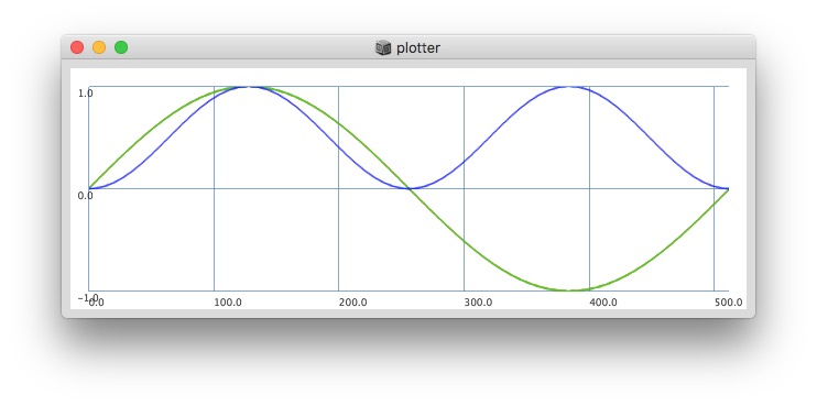
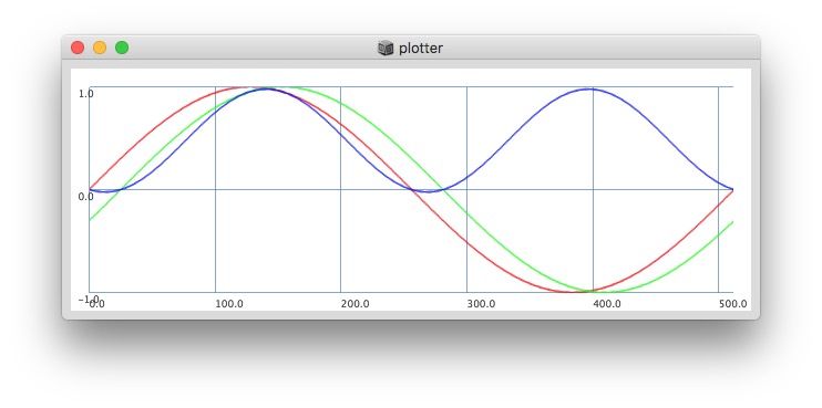
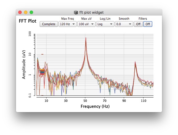
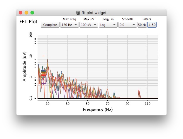
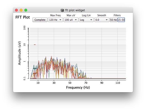
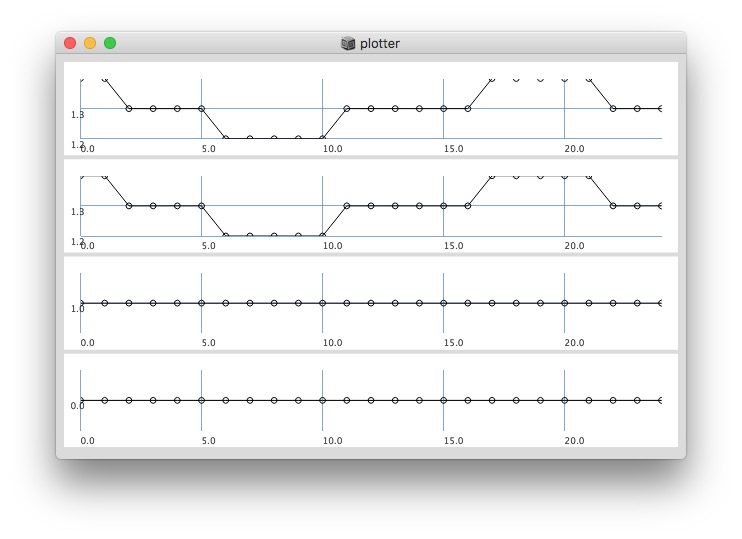
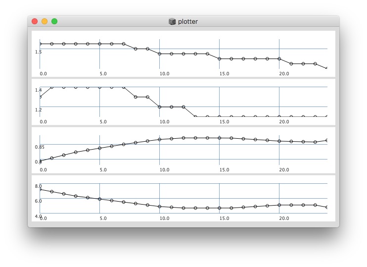
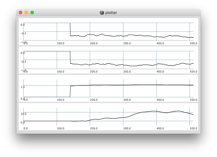
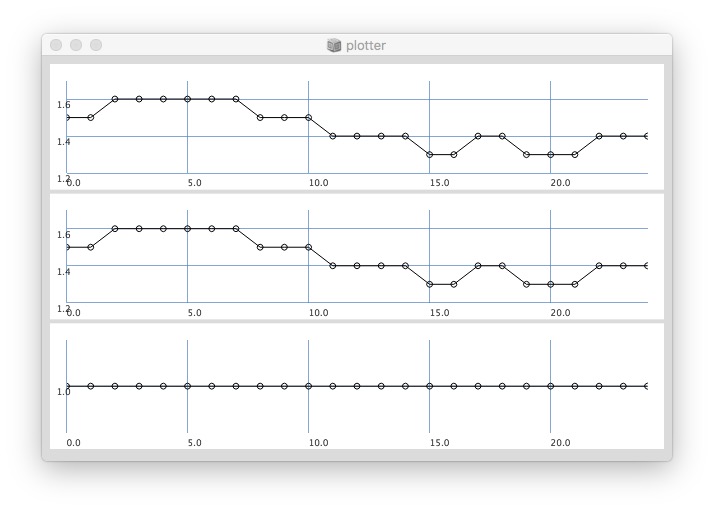
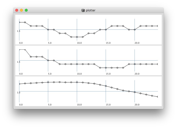
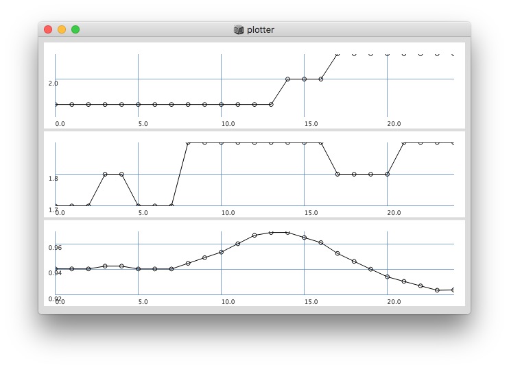
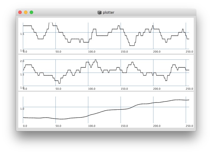
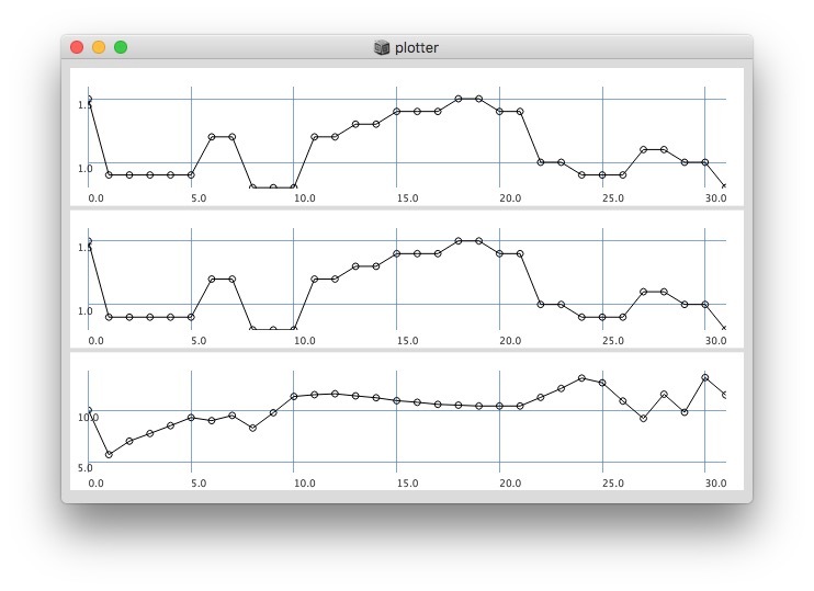
Plotting same signal (~bandEnergyAvg[6]) with 25 and 512 sized window:

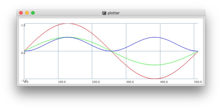
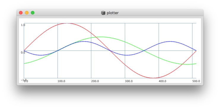
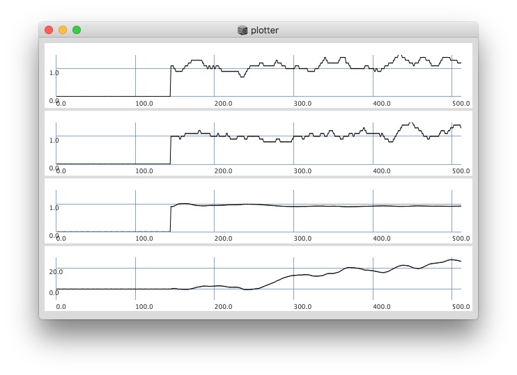
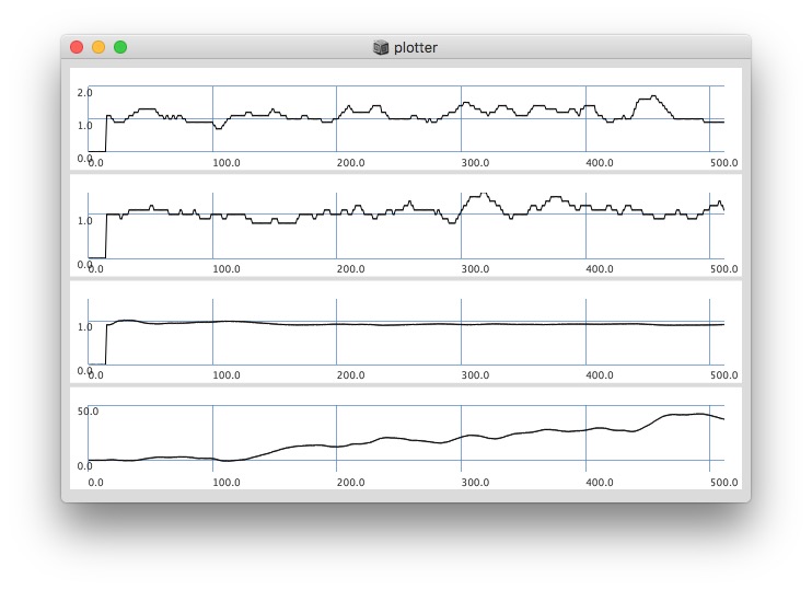
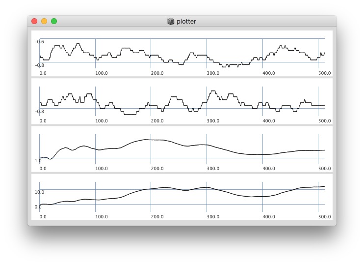
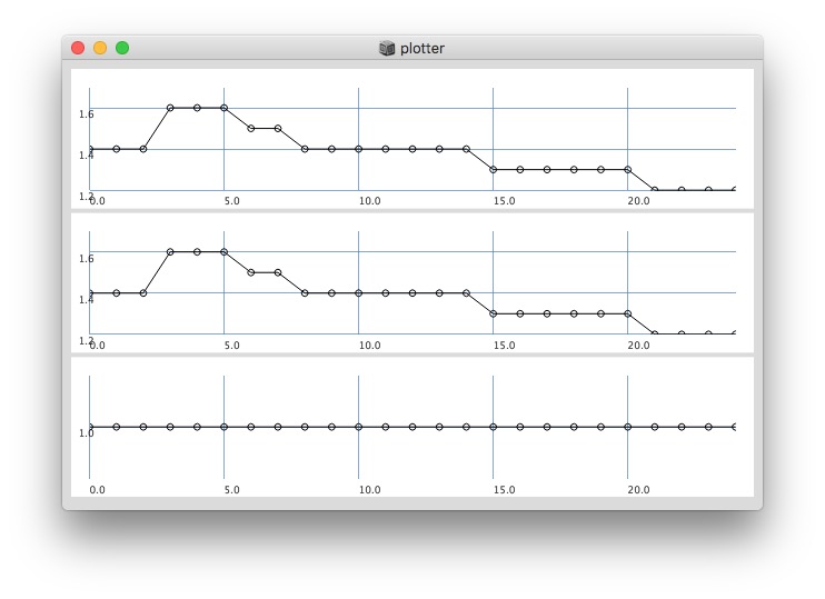
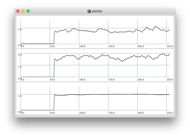
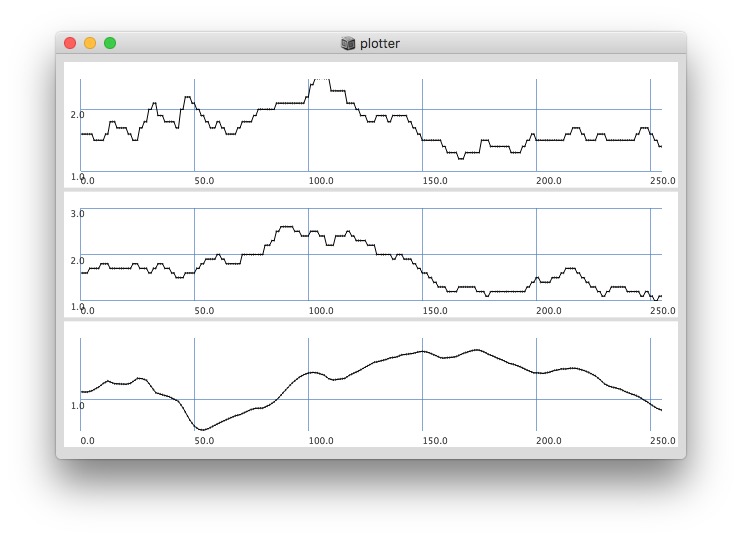
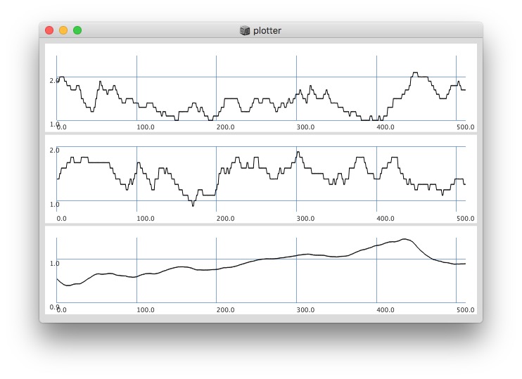
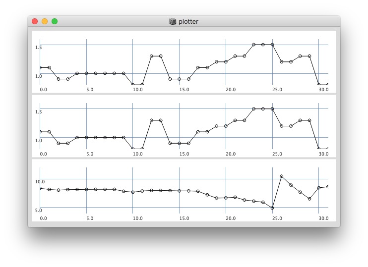
Plotting with different signals (~bandEnergyAvg[6] and ~bandEnergyAvg[7]):

25 sized window:

256 sized window:
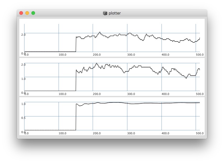
// yes the '0’s at start have an effect on the whole ‘coherence’ plot:

// after '0’s are gone, it changes:

512:

Post window with x, y and a might be interesting as well (512 sized windows):

Signal[ 1.5, 1.5, 1.5, 1.5, 1.5, 1.3999999761581, 1.3999999761581, 1.3999999761581, 1.3999999761581, 1.3999999761581, 1.2999999523163, 1.2999999523163, 1.2000000476837, 1.2000000476837, 1.2000000476837, 1.2000000476837, 1.2000000476837, 1.2000000476837, 1.2000000476837, 1.2000000476837, 1.1000000238419, 1.1000000238419, 1.1000000238419, 1.1000000238419, 1.1000000238419, 1.1000000238419, 1.1000000238419, 1.1000000238419, 1.1000000238419, 1.1000000238419, 1.1000000238419, 1.2000000476837, 1.2000000476837, 1.2...etc...
Signal[ 1.5, 1.3999999761581, 1.3999999761581, 1.2999999523163, 1.2999999523163, 1.3999999761581, 1.3999999761581, 1.3999999761581, 1.2999999523163, 1.2999999523163, 1.2999999523163, 1.2999999523163, 1.2000000476837, 1.2000000476837, 1.1000000238419, 1.1000000238419, 1.2000000476837, 1.2000000476837, 1.2000000476837, 1.2000000476837, 1.2999999523163, 1.2999999523163, 1.2999999523163, 1.2999999523163, 1.2999999523163, 1.2000000476837, 1.2000000476837, 1.2000000476837, 1.2000000476837, 1.2000000476837, 1.2000...etc...
Signal[ 0.98541378974915, 0.98531132936478, 0.98520904779434, 0.98499572277069, 0.98470383882523, 0.98463100194931, 0.98455816507339, 0.98440420627594, 0.98414701223373, 0.98387265205383, 0.9836984872818, 0.98352444171906, 0.98334735631943, 0.9831702709198, 0.98299318552017, 0.98281615972519, 0.98272758722305, 0.98263907432556, 0.98255050182343, 0.98246198892593, 0.98253279924393, 0.98260360956192, 0.98267447948456, 0.98265677690506, 0.98263907432556, 0.98254013061523, 0.98251914978027, 0.98249816894531, 0....etc...
Signal[ 1.5, 1.5, 1.5, 1.5, 1.3999999761581, 1.3999999761581, 1.3999999761581, 1.3999999761581, 1.3999999761581, 1.2999999523163, 1.2999999523163, 1.2000000476837, 1.2000000476837, 1.2000000476837, 1.2000000476837, 1.2000000476837, 1.2000000476837, 1.2000000476837, 1.2000000476837, 1.1000000238419, 1.1000000238419, 1.1000000238419, 1.1000000238419, 1.1000000238419, 1.1000000238419, 1.1000000238419, 1.1000000238419, 1.1000000238419, 1.1000000238419, 1.1000000238419, 1.2000000476837, 1.2000000476837, 1.200000...etc...
Signal[ 1.3999999761581, 1.3999999761581, 1.2999999523163, 1.2999999523163, 1.3999999761581, 1.3999999761581, 1.3999999761581, 1.2999999523163, 1.2999999523163, 1.2999999523163, 1.2999999523163, 1.2000000476837, 1.2000000476837, 1.1000000238419, 1.1000000238419, 1.2000000476837, 1.2000000476837, 1.2000000476837, 1.2000000476837, 1.2999999523163, 1.2999999523163, 1.2999999523163, 1.2999999523163, 1.2999999523163, 1.2000000476837, 1.2000000476837, 1.2000000476837, 1.2000000476837, 1.2000000476837, 1.200000047...etc...
Signal[ 0.98531132936478, 0.98520904779434, 0.98499572277069, 0.98470383882523, 0.98463100194931, 0.98455816507339, 0.98440420627594, 0.98414701223373, 0.98387265205383, 0.9836984872818, 0.98352444171906, 0.98334735631943, 0.9831702709198, 0.98299318552017, 0.98281615972519, 0.98272758722305, 0.98263907432556, 0.98255050182343, 0.98246198892593, 0.98253279924393, 0.98260360956192, 0.98267447948456, 0.98265677690506, 0.98263907432556, 0.98254013061523, 0.98251914978027, 0.98249816894531, 0.98238104581833, 0....etc...
Signal[ 1.5, 1.5, 1.5, 1.3999999761581, 1.3999999761581, 1.3999999761581, 1.3999999761581, 1.3999999761581, 1.2999999523163, 1.2999999523163, 1.2000000476837, 1.2000000476837, 1.2000000476837, 1.2000000476837, 1.2000000476837, 1.2000000476837, 1.2000000476837, 1.2000000476837, 1.1000000238419, 1.1000000238419, 1.1000000238419, 1.1000000238419, 1.1000000238419, 1.1000000238419, 1.1000000238419, 1.1000000238419, 1.1000000238419, 1.1000000238419, 1.1000000238419, 1.2000000476837, 1.2000000476837, 1.20000004768...etc...
Signal[ 1.3999999761581, 1.2999999523163, 1.2999999523163, 1.3999999761581, 1.3999999761581, 1.3999999761581, 1.2999999523163, 1.2999999523163, 1.2999999523163, 1.2999999523163, 1.2000000476837, 1.2000000476837, 1.1000000238419, 1.1000000238419, 1.2000000476837, 1.2000000476837, 1.2000000476837, 1.2000000476837, 1.2999999523163, 1.2999999523163, 1.2999999523163, 1.2999999523163, 1.2999999523163, 1.2000000476837, 1.2000000476837, 1.2000000476837, 1.2000000476837, 1.2000000476837, 1.2000000476837, 1.200000047...etc...
Signal[ 0.98520904779434, 0.98499572277069, 0.98470383882523, 0.98463100194931, 0.98455816507339, 0.98440420627594, 0.98414701223373, 0.98387265205383, 0.9836984872818, 0.98352444171906, 0.98334735631943, 0.9831702709198, 0.98299318552017, 0.98281615972519, 0.98272758722305, 0.98263907432556, 0.98255050182343, 0.98246198892593, 0.98253279924393, 0.98260360956192, 0.98267447948456, 0.98265677690506, 0.98263907432556, 0.98254013061523, 0.98251914978027, 0.98249816894531, 0.98238104581833, 0.9822638630867, 0.9...etc...
Signal[ 1.5, 1.5, 1.3999999761581, 1.3999999761581, 1.3999999761581, 1.3999999761581, 1.3999999761581, 1.2999999523163, 1.2999999523163, 1.2000000476837, 1.2000000476837, 1.2000000476837, 1.2000000476837, 1.2000000476837, 1.2000000476837, 1.2000000476837, 1.2000000476837, 1.1000000238419, 1.1000000238419, 1.1000000238419, 1.1000000238419, 1.1000000238419, 1.1000000238419, 1.1000000238419, 1.1000000238419, 1.1000000238419, 1.1000000238419, 1.1000000238419, 1.2000000476837, 1.2000000476837, 1.2000000476837, 1...etc...
Signal[ 1.2999999523163, 1.2999999523163, 1.3999999761581, 1.3999999761581, 1.3999999761581, 1.2999999523163, 1.2999999523163, 1.2999999523163, 1.2999999523163, 1.2000000476837, 1.2000000476837, 1.1000000238419, 1.1000000238419, 1.2000000476837, 1.2000000476837, 1.2000000476837, 1.2000000476837, 1.2999999523163, 1.2999999523163, 1.2999999523163, 1.2999999523163, 1.2999999523163, 1.2000000476837, 1.2000000476837, 1.2000000476837, 1.2000000476837, 1.2000000476837, 1.2000000476837, 1.2000000476837, 1.200000047...etc...
Signal[ 0.98499572277069, 0.98470383882523, 0.98463100194931, 0.98455816507339, 0.98440420627594, 0.98414701223373, 0.98387265205383, 0.9836984872818, 0.98352444171906, 0.98334735631943, 0.9831702709198, 0.98299318552017, 0.98281615972519, 0.98272758722305, 0.98263907432556, 0.98255050182343, 0.98246198892593, 0.98253279924393, 0.98260360956192, 0.98267447948456, 0.98265677690506, 0.98263907432556, 0.98254013061523, 0.98251914978027, 0.98249816894531, 0.98238104581833, 0.9822638630867, 0.98214656114578, 0.9...etc...
Signal[ 1.5, 1.3999999761581, 1.3999999761581, 1.3999999761581, 1.3999999761581, 1.3999999761581, 1.2999999523163, 1.2999999523163, 1.2000000476837, 1.2000000476837, 1.2000000476837, 1.2000000476837, 1.2000000476837, 1.2000000476837, 1.2000000476837, 1.2000000476837, 1.1000000238419, 1.1000000238419, 1.1000000238419, 1.1000000238419, 1.1000000238419, 1.1000000238419, 1.1000000238419, 1.1000000238419, 1.1000000238419, 1.1000000238419, 1.1000000238419, 1.2000000476837, 1.2000000476837, 1.2000000476837, 1.2000...etc...
Signal[ 1.2999999523163, 1.3999999761581, 1.3999999761581, 1.3999999761581, 1.2999999523163, 1.2999999523163, 1.2999999523163, 1.2999999523163, 1.2000000476837, 1.2000000476837, 1.1000000238419, 1.1000000238419, 1.2000000476837, 1.2000000476837, 1.2000000476837, 1.2000000476837, 1.2999999523163, 1.2999999523163, 1.2999999523163, 1.2999999523163, 1.2999999523163, 1.2000000476837, 1.2000000476837, 1.2000000476837, 1.2000000476837, 1.2000000476837, 1.2000000476837, 1.2000000476837, 1.2000000476837, 1.299999952...etc...
Signal[ 0.98470383882523, 0.98463100194931, 0.98455816507339, 0.98440420627594, 0.98414701223373, 0.98387265205383, 0.9836984872818, 0.98352444171906, 0.98334735631943, 0.9831702709198, 0.98299318552017, 0.98281615972519, 0.98272758722305, 0.98263907432556, 0.98255050182343, 0.98246198892593, 0.98253279924393, 0.98260360956192, 0.98267447948456, 0.98265677690506, 0.98263907432556, 0.98254013061523, 0.98251914978027, 0.98249816894531, 0.98238104581833, 0.9822638630867, 0.98214656114578, 0.98195087909698, 0.9...etc...
Signal[ 1.3999999761581, 1.3999999761581, 1.3999999761581, 1.3999999761581, 1.3999999761581, 1.2999999523163, 1.2999999523163, 1.2000000476837, 1.2000000476837, 1.2000000476837, 1.2000000476837, 1.2000000476837, 1.2000000476837, 1.2000000476837, 1.2000000476837, 1.1000000238419, 1.1000000238419, 1.1000000238419, 1.1000000238419, 1.1000000238419, 1.1000000238419, 1.1000000238419, 1.1000000238419, 1.1000000238419, 1.1000000238419, 1.1000000238419, 1.2000000476837, 1.2000000476837, 1.2000000476837, 1.200000047...etc...
Signal[ 1.3999999761581, 1.3999999761581, 1.3999999761581, 1.2999999523163, 1.2999999523163, 1.2999999523163, 1.2999999523163, 1.2000000476837, 1.2000000476837, 1.1000000238419, 1.1000000238419, 1.2000000476837, 1.2000000476837, 1.2000000476837, 1.2000000476837, 1.2999999523163, 1.2999999523163, 1.2999999523163, 1.2999999523163, 1.2999999523163, 1.2000000476837, 1.2000000476837, 1.2000000476837, 1.2000000476837, 1.2000000476837, 1.2000000476837, 1.2000000476837, 1.2000000476837, 1.2999999523163, 1.299999952...etc...
Signal[ 0.98463100194931, 0.98455816507339, 0.98440420627594, 0.98414701223373, 0.98387265205383, 0.9836984872818, 0.98352444171906, 0.98334735631943, 0.9831702709198, 0.98299318552017, 0.98281615972519, 0.98272758722305, 0.98263907432556, 0.98255050182343, 0.98246198892593, 0.98253279924393, 0.98260360956192, 0.98267447948456, 0.98265677690506, 0.98263907432556, 0.98254013061523, 0.98251914978027, 0.98249816894531, 0.98238104581833, 0.9822638630867, 0.98214656114578, 0.98195087909698, 0.9817550778389, 0.98...etc...
Signal[ 1.3999999761581, 1.3999999761581, 1.3999999761581, 1.3999999761581, 1.2999999523163, 1.2999999523163, 1.2000000476837, 1.2000000476837, 1.2000000476837, 1.2000000476837, 1.2000000476837, 1.2000000476837, 1.2000000476837, 1.2000000476837, 1.1000000238419, 1.1000000238419, 1.1000000238419, 1.1000000238419, 1.1000000238419, 1.1000000238419, 1.1000000238419, 1.1000000238419, 1.1000000238419, 1.1000000238419, 1.1000000238419, 1.2000000476837, 1.2000000476837, 1.2000000476837, 1.2000000476837, 1.200000047...etc...
Signal[ 1.3999999761581, 1.3999999761581, 1.2999999523163, 1.2999999523163, 1.2999999523163, 1.2999999523163, 1.2000000476837, 1.2000000476837, 1.1000000238419, 1.1000000238419, 1.2000000476837, 1.2000000476837, 1.2000000476837, 1.2000000476837, 1.2999999523163, 1.2999999523163, 1.2999999523163, 1.2999999523163, 1.2999999523163, 1.2000000476837, 1.2000000476837, 1.2000000476837, 1.2000000476837, 1.2000000476837, 1.2000000476837, 1.2000000476837, 1.2000000476837, 1.2999999523163, 1.2999999523163, 1.299999952...etc...
Signal[ 0.98455816507339, 0.98440420627594, 0.98414701223373, 0.98387265205383, 0.9836984872818, 0.98352444171906, 0.98334735631943, 0.9831702709198, 0.98299318552017, 0.98281615972519, 0.98272758722305, 0.98263907432556, 0.98255050182343, 0.98246198892593, 0.98253279924393, 0.98260360956192, 0.98267447948456, 0.98265677690506, 0.98263907432556, 0.98254013061523, 0.98251914978027, 0.98249816894531, 0.98238104581833, 0.9822638630867, 0.98214656114578, 0.98195087909698, 0.9817550778389, 0.98157745599747, 0.98...etc...

Many thanks for looking into this… I will carry on thinking…

[jamshark70]

@rodet

b= sum(x*y)/sum(x.squared);

Are those plots based on this line (the last b calculation in your code snippet)? Or based on sum(tempX * tempY)?

If your b calculation is not based on tempX and tempY, then these plots only replicate the previous results. So I still can’t see the result of normalizing and blocking DC.

Thinking a bit further: I’m now fairly sure that dividing by sum(x.squared) is a mistake. The x and y signals should be on equal footing, for one thing. For another, it makes the calculation sensitive to the overall amplitude of x.

f = { |array|
    array = array - array.mean;
    array / array.abs.maxItem;
};

f.(Signal.fill(25, 0).put(10, 1)).squared.sum;
f.(Signal.sineFill(25, [1])).squared.sum;

These two numbers will be very different (first, a single impulse, being lower). So, as the signal becomes more like impulses, sum(tempX.squared) becomes lower and the “correlation” measure rises even if there is no actual correlation between x and y – y could be totally random and this type of change in x would cause so-called correlation to rise. (Note that in your last post, graphs 3 and 4, so-called correlation rises when x drops, and falls when x rises.)

So that’s nonsense.

I was trying to think of a way to control for the amplitudes of x and y, but I think if there is such a way, my math is too limited. I don’t know how to do it. Ask a friend in the math department

But it does seem to me that removing DC and normalizing (as I suggested in the last post) should reduce the impact of the real input data ranges and make the sum dependent on the shapes of the signals rather than their raw amplitudes. This may be valid as a relative measure: “x and y are more correlated now than they were 15 samples ago” but not “x and y are 60% correlated.” Whether this is useful or not, I have no idea.

hjh

[Victor_Bombi]

From the first post it seems that we already have the FFT of EEG signals (not EEG signals), but only for the amplitude component. The “other” component is the phase at every frequency which is missing!!

[jamshark70]

The moving graph looks to me like something produced by the EEG device’s software. But, surely, the device driver is just giving the raw data to client applications…? It’s totally reasonable for the device manufacturer to provide meta-analysis software while also providing lower-level figures.

hjh

[rodet]

@jamshark70

Are those plots based on this line (the last b calculation in your code snippet)? Or based on sum(tempX * tempY)?

If your b calculation is not based on tempX and tempY, then these plots only replicate the previous results. So I still can’t see the result of normalizing and blocking DC.

yes!

I am very sorry, I am an idiot, I left the previous code for b= in the Routine:

b= sum(tempX * tempY) /* /sum(tempX.squared) */;

b= sum(x*y)/sum(x.squared); //this needs to go; 

…

[rodet]

comparing same ~bandEnergyAvg[6] with:

(
var tempX= nil;
var tempY= nil;
x= Signal.newClear(32).fill(0); //change size to 512 for longer window
y= Signal.newClear(32).fill(0); //change size to 512
a= Signal.newClear(32).fill(0); //change size to 512
r= Routine.run({inf.do{
	x= x.rotate(-1);
	y= y.rotate(-1);
	a= a.rotate(-1);
	x[x.size-1]= ~bandEnergyAvg[6];
	y[y.size-1]= ~bandEnergyAvg[6];
	("x:  "++x).postln;
	("y:  "++y).postln;

	// throw away DC (irrelevant to phase)
	tempX = x - x.mean;
	tempY = y - y.mean;
	("tempX-DC:  "++tempX).postln;
	("tempY-DC:  "++tempY).postln;
	
	// normalize after DC removal
	// hope you don't have any all-0 data sets
	tempX = tempX / tempX.abs.maxItem;
	tempY = tempY / tempY.abs.maxItem;
	("tempXnorm: "++tempX).postln;
	("tempYnorm: "++tempY).postln;

	b= sum(tempX * tempY);
	("b:  "++b).postln;
	a[a.size-1]= b;
	("a:  "++a).postln;
	(1/25).wait;
}});
);

r.stop;

(
var data = [x,y,a];
var plotter = Plotter("plotter",Rect(5,5,630,405));
plotter.plotMode = \plines;
plotter.value_(data);
);

post window:

x:  Signal[ 1.2999999523163, 1.2999999523163, 0.80000001192093, 0.80000001192093, 0.89999997615814, 0.89999997615814, 1.1000000238419, 1.1000000238419, 1.2999999523163, 1.2999999523163, 1.2999999523163, 1.2999999523163, 1.2999999523163, 1.0, 1.0, 1.3999999761581, 1.3999999761581, 1.1000000238419, 1.1000000238419, 1.1000000238419, 1.5, 1.5, 1.8999999761581, 1.8999999761581, 1.7999999523163, 1.7999999523163, 2.0, 2.0, 1.7999999523163, 1.7999999523163, 1.7999999523163, 2.2000000476837 ]
y:  Signal[ 1.2999999523163, 1.2999999523163, 0.80000001192093, 0.80000001192093, 0.89999997615814, 0.89999997615814, 1.1000000238419, 1.1000000238419, 1.2999999523163, 1.2999999523163, 1.2999999523163, 1.2999999523163, 1.2999999523163, 1.0, 1.0, 1.3999999761581, 1.3999999761581, 1.1000000238419, 1.1000000238419, 1.1000000238419, 1.5, 1.5, 1.8999999761581, 1.8999999761581, 1.7999999523163, 1.7999999523163, 2.0, 2.0, 1.7999999523163, 1.7999999523163, 1.7999999523163, 2.2000000476837 ]
tempX-DC:  Signal[ -0.10000002384186, -0.10000002384186, -0.59999996423721, -0.59999996423721, -0.5, -0.5, -0.29999995231628, -0.29999995231628, -0.10000002384186, -0.10000002384186, -0.10000002384186, -0.10000002384186, -0.10000002384186, -0.39999997615814, -0.39999997615814, 0.0, 0.0, -0.29999995231628, -0.29999995231628, -0.29999995231628, 0.10000002384186, 0.10000002384186, 0.5, 0.5, 0.39999997615814, 0.39999997615814, 0.60000002384186, 0.60000002384186, 0.39999997615814, 0.39999997615814, 0.39999997615814, 0.8000...etc...
tempY-DC:  Signal[ -0.10000002384186, -0.10000002384186, -0.59999996423721, -0.59999996423721, -0.5, -0.5, -0.29999995231628, -0.29999995231628, -0.10000002384186, -0.10000002384186, -0.10000002384186, -0.10000002384186, -0.10000002384186, -0.39999997615814, -0.39999997615814, 0.0, 0.0, -0.29999995231628, -0.29999995231628, -0.29999995231628, 0.10000002384186, 0.10000002384186, 0.5, 0.5, 0.39999997615814, 0.39999997615814, 0.60000002384186, 0.60000002384186, 0.39999997615814, 0.39999997615814, 0.39999997615814, 0.8000...etc...
tempXnorm: Signal[ -0.12500001490116, -0.12500001490116, -0.74999988079071, -0.74999988079071, -0.62499994039536, -0.62499994039536, -0.37499991059303, -0.37499991059303, -0.12500001490116, -0.12500001490116, -0.12500001490116, -0.12500001490116, -0.12500001490116, -0.49999991059303, -0.49999991059303, 0.0, 0.0, -0.37499991059303, -0.37499991059303, -0.37499991059303, 0.12500001490116, 0.12500001490116, 0.62499994039536, 0.62499994039536, 0.49999991059303, 0.49999991059303, 0.74999994039536, 0.74999994039536, 0.499999...etc...
tempYnorm: Signal[ -0.12500001490116, -0.12500001490116, -0.74999988079071, -0.74999988079071, -0.62499994039536, -0.62499994039536, -0.37499991059303, -0.37499991059303, -0.12500001490116, -0.12500001490116, -0.12500001490116, -0.12500001490116, -0.12500001490116, -0.49999991059303, -0.49999991059303, 0.0, 0.0, -0.37499991059303, -0.37499991059303, -0.37499991059303, 0.12500001490116, 0.12500001490116, 0.62499994039536, 0.62499994039536, 0.49999991059303, 0.49999991059303, 0.74999994039536, 0.74999994039536, 0.499999...etc...
b:  7.4062483943999
a:  Signal[ 5.0161185264587, 5.1491661071777, 5.3056840896606, 5.4379715919495, 5.4111795425415, 5.3712921142578, 5.3712921142578, 5.3712921142578, 5.534704208374, 5.6976256370544, 5.8599395751953, 5.5136227607727, 5.1735763549805, 5.0041151046753, 4.8299250602722, 5.1497669219971, 5.4676218032837, 5.4111771583557, 5.3541402816772, 5.3296194076538, 5.7923603057861, 6.2438831329346, 5.8287601470947, 7.0789575576782, 8.0022201538086, 9.0734615325928, 7.997661113739, 9.4960603713989, 10.353007316589, 10.3530073165...etc...

plotting:

as far as I understand we were hoping for b to be always the same name and therefore a to be represented as a constant line in the third plot.

I am thinking… :

x=[1,2,3,4,5,6,5,4,3,2,1];
y=[1,2,3,4,5,6,5,4,3,2,1];
sum(x*y) // 146
x=[1,2,3,4,5,6,7,6,5,4,3];
y=[1,2,3,4,5,6,7,6,5,4,3];
sum(x*y) //226

so I guess b= sum(tempX * tempY) might be misleading too. But I am still a bit lost here, so it could be that I am talking rubbish.

…

[jamshark70]

Yes, clearly that didn’t work.

I’m out of ideas. But – your loop represents a moving window function, and you’re doing cross-correlation between two signals, so a web search for “cross-correlation moving window” might turn up some algorithms.

Certainly someone has worked on this problem before.

hjh

[rodet]

thanks James, I will meditate a bit and update the thread asap.

cheers! k

[jamshark70]

Hm, after a bit of poking around, I find Pearson’s correlation coefficient might be interesting.

If the data sets have a perfect linear correlation, the coefficient is 1.0. (Perfect negative correlation is -1.0.) 0 is completely decorrelated. “Perfect correlation” does not mean “equal” – x[i] - xMean eliminates DC offset, and the standard deviation product accounts for amplitude differences.

(
f = { |x, y|
	var xMean = x.mean,
	yMean = y.mean,
	momentSum = 0, xDev = 0, yDev = 0;
	
	x.size.do { |i|
		var xDiff = (x[i] - xMean),
		yDiff = (y[i] - yMean);
		momentSum = momentSum + (xDiff * yDiff);
		xDev = xDev + xDiff.squared;
		yDev = yDev + yDiff.squared;
	};
	xDev = (xDev / (x.size - 1)).sqrt;
	yDev = (yDev / (x.size - 1)).sqrt;  // if y has extra items, they're ignored
	
	momentSum / ((x.size - 1) * xDev * yDev)
};
)

f.(x, x);  // equal datasets
-> 1.0

f.(x, x * 3 + 0.5);  // in phase but different amplitude + DC
-> 1.0

f.(x, x.rotate(20));  // out of phase
-> 0.5555702330196

Edit: The formula is sigma[i = 0…n-1]((x[i] - xMean) * (y[i] - yMean)) / ((n-1) * stdev(x) * stdev(y)) … (x[i] - xMean) matches x - xMean in my original attempt, meaning that the top of the fraction is actually a sum(x * y) with an adjustment for DC. So I’d guessed that part right. What we were missing was the correction for amplitude, which Pearson provides with the product of standard deviations.

hjh