How to implement auto gain

[Thor_Madsen]

I have been messing around with @nathan s negative compression code, really cool stuff. Read more here. I was happy to read the explanation of why Compander doesn’t really work for short attack and release time (downsampling the input for detection) as this has been my own experience too, without knowing why.

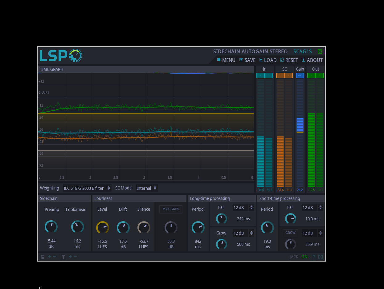
Usually when I work with compression in a DAW context I don’t use autogain, instead I prefer setting the makeup gain manually. However, there are a couple of situations where autogain would be a nice feature to implement. First one is expansion (corresponding to slope > 1 in Nathan’s code, where slope is the reciprocal of ratio), since expansion has the potential for making the output extremely loud. Another case would be an ‘intelligent’ compressor which compresses the input material based on the loudness of the signal so that even very dynamic material will receive (close to) the same amount of compression - there are commercial plugins doing this already, can’t think of the names right now. This is useful for applying compression as an ‘envelope shaper’ on very dynamic material rather than just a way of controlling dynamics.

So how do you best implement autogain? I suppose you need to calculate the RMS which will either introduce latency or mean than the detection of sudden changes in the dynamics of the input signal will be delayed by the RMS window size. Is there a way to implement autogain (maybe not in a ‘perfect’ way) without introducing additional latency in the signal chain?

[smoge]

There is an LSP (freesoftware / linux) plugin called “autogain sideline”. Without a lookahead it is difficult to have a good result, so there is at least 50-400ms. It also has an input for a “sideline” signal, I imagine to serve as reference. Maybe you can play with it and see if that’s it or something else?

Will that be it?

https://lsp-plug.in/?page=manuals&section=sc_autogain_stereo

This plugin provides automatic gain control tools that support loudness matching according to the ITU-R BS.1770-4 recommendation. That means that the input signal is being processed via the weighting filter (K-filter) before the measurement of it’s energy is performed. According to the BS.1770-4 recommendation, the energy measurement period should be of 400 milliseconds but the plugin allows to vary this value. As an additional option, it also provides other kind of weighting filters provided by the the IEC 61672:2003 standard: A, B, C and D weighting filters.

Additional sidechain input allows to gain the control over the loudness of the output in two different modes:

• Control

• the loudness level of the sidechain signal is measured, then the corresponding gain correction is computed to match the loudness of the sidechain signal to the desired loudness level, and the computed gain is applied to the original track.* Match
• the loudness level of the sidechain signal is measured, then the measured loudness is interpreted as a desired loudness level. After that, the loudness of the input signal is measured, then the corresponding gain correction is computed to match the loudness level of the input signal to the loudness level of the sidechain signal.

If the level of the signal rapidly changes, the plugin can also rapidly reduce the shocking effect of the loud sound and (if enabled) rapidly raise the gain, too. Despite, because it uses RMS measurements, it does not fully protect from sudden loud clicks/pops, and aditional surge protection should be applied. Additional control over the zero level also makes the plugin act as a trigger: if the signal is below the mimum level, then the gain value does not change. This prevents from significant amplification of a background noise in the case of long silence at the input.

[smoge]

Are you trying to implement something like this in SC? The plugin seems to take care of a lot of things at the same time to be more or less convincing, mixing different techniques etc

LSP plugins are also JACK standalone apps, so you can use as a insert in sc… ?

[nathan]

I have never heard the term “autogain,” but a cursory search tells me that it’s another term for “makeup gain.” Is this true?

Makeup gain is straightforward to implement. Pick a reference amplitude in dB and run it through the gain control formula:

referenceAmplitudeDb = 0.0;
referenceAmplitudePredicted = ((referenceAmplitudeDb - threshold).max(0) * (slope - 1)).lag(attack).dbamp;
makeupGain = 1 / referenceAmplitudePredicted;

Then just multiply this by the output of the compressor.

However, two caveats to be aware of: 1. makeup gain as I have implemented it here is a blunt instrument, it doesn’t normalize loudness. I think this is the case for the makeup gain control in most compressors in the biz. 2. The fact that my code could be used as an expander doesn’t mean that it should. I avoided talking about expanders much because they have different aesthetic goals from compressors and demand a different design approach.

The “intelligent compression” you describe, based on loudness normalization, is a different concept from makeup gain. (I think? I don’t know, the terminology in this space is very confused.) It can be implemented by using a second compressor with much slower settings. The topology would be something like: slow compressor → fast compressor → divide by the gain of the slower compressor.

I should mention that while I may look knowledgeable about the math of compressors, I’ve never actually gone through the process of developing one and trying to optimize it for the best sound, so I’m not really a compression expert or anything, just an ideas guy.

[Thor_Madsen]

@nathan - I adopted the term autogain (or rather Auto Gain) from Logic X to mean automatic makeup gain. Going back to your compressor code - I think it works great and I like the way four different types of dynamic control can all be obtain from the same simple formula - normal downward compression with any ratio (or slope), brickwall limiting, upward expansion and (brand new to me) negative compression. Both normal downward compression and negative compression sound quite good on guitar and others signals, like beats and bass, and better than Compander to my ears. I will keep experimenting. One question: how do you change the knee?

[Thor_Madsen]

This looks interesting, I am on OSX, now would you connect sc to the plugin?

[jamshark70]

It’s perhaps a naive approach, but when I got tired of distortion getting louder at higher gain, I did this:

// hjh 2022 - gplv3

ConstantGainDistortion {
	*ar { |in, preamp = 1, distFunc(_.tanh), rmsSize = 512|
		var distorted = distFunc.value(in * preamp);

		var ampBefore = (RunningSum.ar(in.squared.asArray.sum, rmsSize) / rmsSize).sqrt;
		var ampAfter = (RunningSum.ar(distorted.squared.asArray.sum, rmsSize) / rmsSize).sqrt;

		^distorted * min(10, (ampBefore / max(0.01, ampAfter)))
	}

	*kr { |in, preamp = 1, distFunc(_.tanh), rmsSize = 512|
		var distorted = distFunc.value(in * preamp);
		var size = rmsSize / BlockSize.ir;

		var ampBefore = (RunningSum.kr(in.squared.asArray.sum, size) / size).sqrt;
		var ampAfter = (RunningSum.kr(distorted.squared.asArray.sum, size) / size).sqrt;

		^distorted * min(10, (ampBefore / max(0.01, ampAfter)))
	}
}

distFunc could be a compressor too.

It’s not exactly constant gain, but if I do (SinOsc.ar(110) * preamp.dbamp).tanh and vary preamp between -20 and 40 dB, the 512-point RMS of the raw tanh ranges -23 to 0 dB (approximately), while the ConstantGainDistortion output ranges -3.26 to -2.97 dB. Y’know, I’ll take it.

I use this a lot for notes with relatively static dynamics. I haven’t tried this for auto-makeup gain on drums, but I’d expect a poor result because of the rapid envelopes. (Come to think of it, it would be nonsense to match a compressor’s output to the input’s envelope, since the whole point of drum compression is to smooth out the envelope a bit.)

@Thor_Madsen

This looks interesting, I am on OSX, now would you connect sc to the plugin?

The “Linux Studio Plugins” project appears not to place MacOS support as a high priority – i.e., at their official download page, you can find Linux and FreeBSD binaries, and that’s it.

The site’s main page says “The basic idea is to fill the lack of good and useful plugins under the GNU/Linux platform,” so I think their idea is, if you’re on Mac or Windows, there are already plenty of plug-ins.

The page also claims to support the LinuxVST plug-in format, but unfortunately, the SC VSTPlugin UGen doesn’t recognize them. AFAICS the only way in Linux is as smoge said – to use JACK ports as an outboard insert.

hjh

[Thor_Madsen]

I was playing around with RunningSum after seeing your post on the FB page and also comparing it to FluidLoudness, but methods yielded good results. What is the idea of, or math behind squaring and square rooting the signal?

(Come to think of it, it would be nonsense to match a compressor’s output to the input’s envelope, since the whole point of drum compression is to smooth out the envelope a bit.)

I was thinking more in terms of auto gain with expansion which can be interesting on percussion and sometimes I will use it if I get some material which is over compressed to begin with.

[Thor_Madsen]

Negative expansion. Haven’t really tested it yet but I think it would be nice a sustain fx on piano or guitar like instruments with a long natural decay.

(
{
	var thresh = -6;
	var slope = -0.5; 
	var atk = 0.05;
	var rel = 0.2;
	var floor = -40;
	var sig = SinOsc.ar(440) * Env.perc(0.3, 0.6, 0.1, -4).ar(2);
	var cres = Slope.ar(Slope.ar(sig)) > 0;
	var max = RunningMax.ar(sig).ampdb;
	var amplitude = Amplitude.ar(sig, atk, rel).ampdb;
	var gain = ((amplitude - max - thresh).min(0) * (slope - 1) * (amplitude > floor)).lag(0.1).dbamp;
	[sig, sig * gain]
}.plot(1);
)

[jamshark70]

@Thor_Madsen

What is the idea of, or math behind squaring and square rooting the signal?

It’s just the standard RMS formula (square Root of the Mean of the Squared sample values).

I don’t have a formal understanding of the rationale, but I could intuitively, right-brainily speculate: If you have two values, a and b, then the square root of the sum of the squares is the distance from the origin, in two dimensions. If you have 3 values, sqrt(x^2 + y^2 + z^2) is the distance in 3 dimensions. So n values would give the n-dimensional distance. The “mean” part divides by a constant, so RMS is proportional to the n-dimensional distance. (If that’s too confusing: squaring the samples ensures all positive values, and the square root at the end “undoes” the squaring, though it isn’t the same as the sum of the samples, think Pythagorean theorem.)

hjh

[Thor_Madsen]

I worked some more on it

(
f = {
	var thresh = -6;
	var range = 24; // dynamic range in dB
	var atk = 0.02;
	var rel = 0.02;
	var noisefloor = -70;	
	var sig = LFSaw.ar(440) * Env.perc(0.1, 0.6, LFPulse.ar(1).range(0.05, 0.4), -4).ar(0, Impulse.ar(1));
	var amplitude = Amplitude.ar(sig, atk, rel).ampdb;
	var max = Peak.ar(sig, amplitude < noisefloor).ampdb;
	var floor = max + thresh - range;
	var gain0 = ((amplitude - max - thresh).min(0) * (0.25 - 1) * (amplitude > floor)  ).dbamp;
	var gain1 = ((amplitude - max - thresh).min(0) * (0 - 1) * (amplitude > floor)  ).dbamp;
	var gain2 = ((amplitude - max - thresh).min(0) * (-0.5 - 1) * (amplitude > floor)  ).dbamp;
	[sig, sig * gain0.lag(0.2), sig * gain1.lag(0.2), sig * gain2.lag(0.2) ]; 
	// [sig, sig * gain0.lag(0.2)] // uncomment and uncomment f.play below to listen
	// [sig, sig * gain1.lag(0.2)] // do.
	// [sig, sig * gain2.lag(0.2)] // do.
};
f.plot(2)
// f.play
)

The above code produces the plot below, which show (top to bottom): original signal, expansion with a 0.25 slope (4:1 ratio), expansion with a slope of 0 (brickwall) and -0.5 (negative expansion). Expansion kicks in when the signal drops 6 db below ‘max’ which is the peak level of the signal since last silence and is released when the signal drops below the floor, which is defined as max + thresh - range. So in other words, the dynamic range is static but the ceiling and floor of the dynamic operation depends on the peak of the signal.

[smoge]

@Thor_Madsen

This looks interesting, I am on OSX, now would you connect sc to the plugin?

You can do this, in the same way that SC can be an insert in an Ardour track(s). JACK allows this type of patching between programs, that’s something good about linux that macos doesn’t offer.

I’m not exactly sure how this reflects in terms of processing parallelism. As far as I know, Ardour will take care of that when possible, not sure about standalone jack apps connected to scsynth. Jack2 offers multi-core parallelism, but would need to check how that works in different cases.

[nathan]

@Thor_Madsen

Going back to your compressor code - I think it works great and I like the way four different types of dynamic control can all be obtain from the same simple formula - normal downward compression with any ratio (or slope), brickwall limiting, upward expansion and (brand new to me) negative compression. Both normal downward compression and negative compression sound quite good on guitar and others signals, like beats and bass, and better than Compander to my ears. I will keep experimenting. One question: how do you change the knee?

The code was written just as a minimum working demo of negative compression that also avoids the design mistake in Compander, it’s not meant to be a professional-quality compressor. Compression, limiting, and expansion have different aesthetic goals, so the idea of using the same math for all three has some limitations to me. More important than mathematical consistency is the sound.

There’s lots more to compressor design than the textbook algorithms I presented — soft knee, lookahead, true peak, brickwalling, program dependence, feedback/feedforward topologies, concave compression, multichannel considerations, tons of weird virtual analog inside baseball too. I do plan on writing more about these but I don’t feel qualified to do so quite yet, as I only understand them on paper, not in the studio.

---

There’s some confusion here about RMS. From the name RMS, it’s often assumed that it’s literally taking the root, mean, and square of finite chunks of samples. This isn’t inaccurate, but it’s a narrower definition than is actually used in practical compressor design.

RMS broadly refers to any signal chain comprising x^2, then lowpassing, then sqrt. A lowpass filter with an impulse response that is non-oscillatory and a sum/integral of 1 is a weighted mean. (The sum/integral being 1 can be ignored if the definition of “mean” is relaxed.) So just writing x.squared.lag(0.1).sqrt computes RMS. You will get different results from, say, x.abs.lag(0.1), which is a more typical (symmetrical) envelope follower using full-wave rectification (abs). The “sliding finite window” view of RMS is a variant where the lowpass is an FIR filter, often computed in a downsampled manner, but it’s not the only way to do it. You can use IIR filters too. IIR RMS implementations have been used in analog circuits since the 70’s.

RMS is less reactive to sudden transients than full-wave rectification, even if both kinds of envelope followers are tuned to the same attack/release settings. For this reason, it’s a good choice if you have a long attack/release and want to get a baseline to compare transients to. A lot of loudness standards like LUFS employ this idea (and do use FIR sliding windows).

RMS comes from EE, where it has an important property that if you have two signals A and B that are statistically uncorrelated with each other, then the RMS of the summed signals is RMS(A+B) = sqrt(RMS(A)^2 + RMS(B)^2). I don’t remember off the top of my head if there’s an equivalent for full-wave rectification.

[smoge]

@nathan

There’s some confusion here about RMS. From the name RMS, it’s often assumed that it’s literally taking the root, mean, and square of finite chunks of samples. This isn’t inaccurate, but it’s a narrower definition than is actually used in practical compressor design.

Interesting. But x also has an accumulator, right? It’s like a fold. How much does the size of the “window” influence it? How helpful are RMS of very short duration? We could measure RMS in very different ways, from short windows to continuously calculation using the accumulated sum of squares and the number of samples in a longer duration. In this case, it is a bit helpless with sudden changes, right? The LSP plugin choose to use both short- and long-“time processing”

I have used this code bellow, defined as a foldr, maybe you can find something wrong with it. Let me know.

rms samples = sqrt (foldr (\sample acc -> acc + sample^2) 0 samples / length samples)

[prko]

The sound quality is not so good, but I would like to share my simple experience with Normaliser (Input → Normaliser → Amplitude automation):

(
{
	var source, inputAmplitude, autoAmplitude, normalised, out;
	source = LFPulse.ar * 0.1;
	inputAmplitude = LFNoise2.ar(LFSaw.kr(1).range(1, 100)).range(0, 0.2);
	autoAmplitude = SinOsc.kr(10).range(0.01, 0.2);
	normalised = Normalizer.ar(source * inputAmplitude, 0.1, 0.004); // scaling to adjust vertical range
	out = normalised * autoAmplitude * 10; // rescaling
	[source, inputAmplitude, autoAmplitude, normalised, out]
}.plot(0.5)
)

(
x = {
	var source, inputAmplitude, autoAmplitude, out;
	source = SinOsc.ar * 0.1;
	inputAmplitude = LFNoise2.ar(LFSaw.kr(1).range(1, 100)).range(0, 0.2);
	autoAmplitude = SinOsc.ar(1).range(0.01, 0.2);
	Normalizer.ar(source * inputAmplitude, autoAmplitude, 0.004)
}.play
)

[Thor_Madsen]

@nathan - looking forward to more writings about compressors on your blog. One of my favorite hardware compressors is the LA2A - it almost impossible to get ‘bad compression’ with a LA2A unlike most other compressors. The UAD LA2A plugin is very close to the hardware (I got both), I probably couldn’t tell them apart in an AB test. If you ever felt like taking about the LA2A and possibly emulate some aspects of it in SC I would be very interested. I have tried to find sources explaining how it works but I still don’t really understand in which way it is program dependent and how the ratios are derived.

[nathan]

The LA2A’s schematics are out here:

Teletronix%20Model%20LA-2A%20Leveling%20Amplifier.pdf

This 1966 patent too:

https://patents.google.com/patent/US3258707A/en?oq=3258707

The actual topology of it is a fairly standard feedforward opto compressor, but it’s all in the details. Aside from the components all being carefully tuned, opto cells do some really weird things. To emulate it I’d need a year where I don’t work on anything else (and get cadmium poisoning from experimenting with photoresistors, but I don’t mind suffering for art).

[Thor_Madsen]

haha, yea I figured it wasn’t that easy