Understanding Resonz

I’m trying to wrap my head around the specifics of Resonz.

The paper linked in the help file concludes that the filter should have constant gain with respect to frequency; but I believe this would mean keeping bw constant, which means supercollider’s parameter bwr would have to move in inverse proportion to freq, in order to keep bw and therefore gain constant.

I’m finding the documentation a little thin. Maybe I’m missing something. The .cpp code is also uncommented. I’ve been looking at pages with all these equations but unfortunately that’s not my forte. Wherever I start reading they seem to have defined some of the variables on a previous page and I’m not ready to dig into a textbook from page one… All I’m trying to do is plot freq vs magnitude response given (constant) params freq and bw! Anyone have a good grasp of this stuff?

I’m not sure what the author of Resonz was getting at either. It doesn’t quite line up with the paper from what I see, but I can derive the filter magnitude response for you with some help from the Z-transform.

Filter coefficient code (from FilterUGens.cpp):

        double ffreq = freq * unit->mRate->mRadiansPerSample;
        double B = ffreq * rq;
        double R = 1.f - B * 0.5f;
        double twoR = 2.f * R;
        double R2 = R * R;
        double cost = (twoR * cos(ffreq)) / (1.f + R2);
        double b1_next = twoR * cost;
        double b2_next = -R2;
        double a0_next = (1.f - R2) * 0.5f;

Cleaned up:

theta = freq * 2pi / sampleRate;
R = 1 - (theta * rq)/2;
b1 = (4 R^2 cos(theta)) / (1 + R^2);
b2 = -R^2;
a0 = (1 - R^2) / 2;

Filter update code:

y0 = ZXP(in) + b1 * y1 + b2 * y2; ZXP(out) = a0 * (y0 - y2);

De-obfuscated:

w[t] = x[t] + b1 * w[t-1] + b2 * w[t-2]
y[t] = a0 * (w[t] - w[t - 2]);

So we’re looking at a Direct Form II implementation of the following filter, here using capital letters to distinguish from the code:

H(z) = (B0 + B1 z^-1 + B2 z^-2) / (A0 + A1 z^-1 + A2 z^-2)

A0 = 1
A1 = -b1
A2 = -b2
B0 = a0
B1 = 0
B2 = -a0

To derive the magnitude response at frequency f, let omega = f * 2pi / sampleRate. Then the gain as a function of omega is:

G(omega) = |H(e^(omega * j))|

where j is the imaginary constant.

Here’s some Python/NumPy/Matplotlib code to plot the frequency response:

import numpy as np
import matplotlib.pyplot as plt

sample_rate = 48000

def plot_resonz_magnitude_response(filter_frequency, rq):
    theta = filter_frequency * 2 * np.pi / sample_rate
    R = 1 - (theta * rq) / 2
    b1 = (4 * R * R * np.cos(theta)) / (1 + R * R)
    b2 = -R * R;
    a0 = (1 - R * R) / 2

    A0 = 1
    A1 = -b1
    A2 = -b2
    B0 = a0
    B1 = 0
    B2 = -a0

    frequency = np.linspace(0, sample_rate / 2, 10000)
    omega = frequency * 2 * np.pi / sample_rate
    z = np.exp(omega * 1j)
    z1 = 1 / z
    z2 = 1 / (z * z)
    H = (B0 + B1 * z1 + B2 * z2) / (A0 + A1 * z1 + A2 * z2)
    G = np.abs(H)

    plt.plot(frequency, 20 * np.log10(G))

plt.ylim(-60, 10)
plt.xlabel("Frequency (Hz)")
plt.ylabel("Magnitude (dB)")

for filter_frequency in np.linspace(100, 10000, 10):
    plot_resonz_magnitude_response(filter_frequency, rq=0.1)

plt.savefig("resonz.png")

This plots a few Resonz frequency responses from 100 Hz to 10 kHz, all with rq set to 0.1:

resonz

Although I could have made a mistake somewhere, the results at least look correct.

7 Likes

Wow Nathan, that’s amazingly helpful and detailed. I’m very grateful!

Should the ffreq in the second code-block be theta?

The H(z) equation was derived from the code? Or that’s a textbook formula for this kind of filter? I didn’t see the H(z) equation on the “Direct Form II” link, and it’s not clear to me how we know that the Resonz filter implements “Direct Form II”, since the y(t) equation looks to be different.


To make things a little more interesting: I noticed that csound also has a resonz, which has more extensive documentation, but which may or may not be the same as our Resonz. Digging into their doc, I found that Stiglitz defines the H(z) equation for csound-Resonz as (1 - z^-2) / (1 - 2Rcos(theta)z^-1 + R^2z^-2).

I subbed this into your python code and noticed that it doesn’t give the same curves as your H, and that the curves do NOT have constant gain.

H = (1 - z2) / (1 - (2 * R * np.cos(theta) * z1) + (R * R * z2))
resonz1

HOWEVER, when I changed rq to vary with filter_frequency, so as to preserve constant bw, the curves then had constant gain.

plot_resonz_magnitude_response(filter_frequency, rq=(10 / filter_frequency))
resonz2

So your equation for Resonz has constant gain with constant rq, wheras csound-Resonz has constant gain with constant bw.

If my arithmetic scribblings are correct, though, rq would be more musically useful because it scales the bandwidth to something more like (but not exactly like) the pitch relation rather than the frequency relation.

The curves for csound-Resonz also seem to be taller on the magnitude axis, but I’m not sure whether this is significant.

… I’m rethinking the statement that constant rq is necesarily more musically useful than constant bw…

say we have input ideal white noise, and we want to keep output amp constant while moving the frequency, then we need to keep the integral constant, i.e. the area under the peak, not the peak height. so maybe a set of curves more like the csound-Resonz ones is better for that?

Looking at Ringz, I see it says it is like Resonz with “constant skirt” rather than constant gain – perhaps that’s the same as csound-Resonz? Does “constant skirt” imply constant amplitude output as in the ideal example above?

Of course, Ringz does not specify bw or rq, but rather decaytime – the doc says decaytime specifies bandwidth but doesn’t mention exactly how. I’m sure a little dive into the .cpp will turn this relation up without too much trouble, which I will do later and post it here (and I imagine it should be added to the doc as well…)

1 Like

You’re welcome! Fixed the ffreq/theta error, thanks for the note.

The H(z) equation is the general form of a second-order digital IIR filter, which is also the general form of a second-order rational function in z^-1.

The y[t] formula matches the second Direct Form II equation if you distribute the multiplication like so: y[t] = a0 * w[t] + 0 * w[t - 1] - a0 * w[t - 2].

I think you’re missing the leading “G” term described in the paper, which does the amplitude compensation.

1 Like

and so pretty!

.
.
.

You’re right, I’m missing the gain factor – I was looking in the textbook, not the article.

Aside from the gain factor, there is another slight difference in the equations between Stieglitz’ book and article. The book has numerator 1 - z^-2 while the article has 1 - Rz^-2. This doesn’t seem to have to do with the gain factor, and seems to have very little difference on the shape of the curves. Neither one of these quite seems identical to the equation you’ve given, but again, there is no(?) difference in the curves.

Once I added the gain factor in, csound-resonz seems to be the same as our resonz.

1 Like

The only differences I can see between the code of Resonz and Ringz are as follows:

Ringz has R = exp(log001 / (decayTime * SAMPLERATE)
Resonz R = 1 - B * 0.5 [ B is bandwidth ]

Ringz has a0 = 0.5
Resonz a0 = (1 - R2) * 0.5 [ this is the scaling factor ]

modifying the python code to plot it:

import numpy as np
import matplotlib.pyplot as plt

sample_rate = 48000

def plot_ringz_magnitude_response(filter_frequency, decay_time):
    theta = filter_frequency * 2 * np.pi / sample_rate
    #R = 1 - (theta * rq) / 2 #resonz version
    R = np.exp(np.log(0.001) / (decay_time * sample_rate))
    b1 = (4 * R * R * np.cos(theta)) / (1 + R * R)
    b2 = -R * R;
    #a0 = (1 - R * R) / 2 # resonz version
    a0 = 0.5
    A0 = 1
    A1 = -b1
    A2 = -b2
    B0 = a0
    B1 = 0
    B2 = -a0

    frequency = np.linspace(0, sample_rate / 2, 50000)
    omega = frequency * 2 * np.pi / sample_rate
    z = np.exp(omega * 1j)
    z1 = 1 / z
    z2 = 1 / (z * z)
    H = (B0 + B1 * z1 + B2 * z2) / (A0 + A1 * z1 + A2 * z2)
    G = np.abs(H)

    plt.plot(frequency, 20 * np.log10(G))

plt.ylim(-60, 100)
plt.xlabel("Frequency (Hz)")
plt.ylabel("Magnitude (dB)")

for filter_frequency in np.linspace(100, 10000, 10):
    plot_ringz_magnitude_response(filter_frequency, decay_time=1)

plt.savefig("ringz.png")

ringz

We can see gains are high and equal, bandwidths are equal. changing decay_time to something very small makes the bandwidth wider and the gain lower.

1 Like

If anyone can work out the relation between bandwidth and decay_time, i’d find that interesting…

1 Like

This is a tricky question, and I haven’t found an existing resource that talks about ring time. We’ll have to derive it ourselves.

Consider the all-pole filter H(z) = G 1 / (1 - 2Rcos(theta)z^-1 + R^2z^-2), where the zeros have been removed and the numerator is now 1 (zeros are roots of the numerator polynomial in z, poles are roots of the denominator polynomial). I believe the impulse response of this filter is of the form h[t] = A cos(phi*t) e^(-kt), where A is a constant gain, phi is the ringing frequency, and k is a positive constant that controls the decay time. The -60 dB ring time of this filter is found by setting e^(-k t_60) = 0.001 => or t_60 = -ln(0.001)/k. Take the z-transform of h[t] (use the formula on Wikipedia) and try to match the coefficients with those of the denominator of H(z). This should give you t_60 in terms of R. I think you’ll get theta = phi also.

To derive bandwidth, make sure your peak amplitude is normalized to 1 and then solve the equation |H(e^(j omega))| = 1 / sqrt(2) in terms of omega. This looks hard but note that |H(e^(j omega))|^2 = 1 / 2 and |G / (a + bj)|^2 = G^2 / (a^2 + b^2) for real a and b so this boils down to separating the real and imaginary parts of the denominator polynomial. I think ultimately you’ll get a polynomial which has two roots, corresponding to the 1 / sqrt(2) point to the left and the right of theta. These should be even distances from theta, and that distance is the bandwidth.

Adding the zeros back in, H(z) = G (1 - z^-2) / (1 - 2Rcos(theta)z^-1 + R^2z^-2) is the equivalent of convolving the all-pole filter impulse response with a 2nd-order FIR filter (in this case subtracting a 2-sample-delay from the dry signal). So I guess I would define ring time of such a filter as being the same as the all-pole case. You could probably get away with defining the bandwidth as being the same as the all-pole case also, even though the 1 / sqrt(2) equality is no longer strictly correct.

I can’t do the full derivation right now but hopefully these sketched-out steps will give you an idea. There may be mistakes in the above. Let me know if you have questions.

1 Like

OK, wow. Thanks very much for that, Nathan. I’m a little over my head with this right now, unfortunately. I’m going to have to step back quite a few steps to understand this kind of stuff. I appreciate a lot that you seem to be up for discussing these issues, and I hope to take you up on it more in the future :slight_smile:

Personally it looks like I have to follow two tracks, one to really understand the meaning of the math and how dsp really works, and the other just to use these things programatically with a good understanding of what’s going to happen. Thinking of the Resonz filter as a black-box function, seems to me like there’s a gap where either it must be used “by hand” or really understood on an engineering level. As someone who wants to program with it, I was expecting it to behave like a code library (and be documented like one), and found it a rather odd beast. I’m horrified and fascinated…


Ok, back to some details:

I think that where Ringz and Resonz are concerned, to compute the relationship between ringtime and bandwidth, we can use the approximate definition for bandwidth as defined in the code Resonz, and get

R = 1 - B/2 and R = e^(log001 / (decaytime * samplerate))

… so the relationship is dependent on samplerate, but if we solve for rq instead of B then it’s dependent on freq but not samplerate…


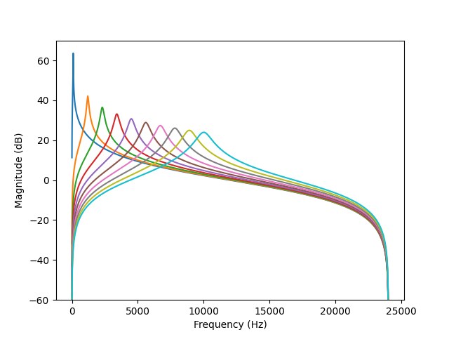
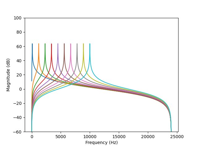
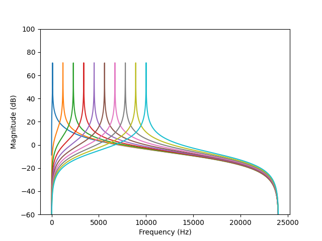
I was also trying to figure out the scaling stuff – I really wanted to have control over the output amp, not the peak gain, and it looks like the scaling factor should be sqrt(a0) rather than our a0 (for peak gain). This is both in the Stieglitz paper and csound’s version of resonz. a0 = (1 - R * R) / 2

This scaling doesn’t set amplitude to one however, they’re still too high. But it’s a good start as once it’s multiplied by sqrt(a0) rather than a0, we can just use another constant scalar rather than one that’s dependent on the parameters. The claim in the literature is that it sets the RMS to one but I don’t think I’m getting this.

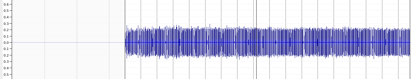
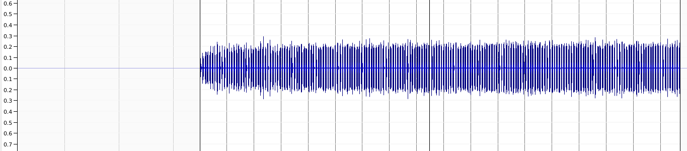
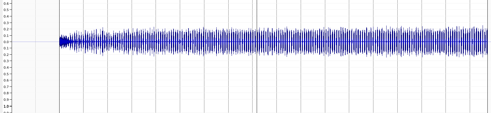
sqrt(a0) experimentally results in amplitudes that are almost constant across much of the frequency range, but low frequencies with skinny bandwidths are still lower in amp – I suppose this is to be expected because there’s less time to express the frequency? I mention it because one might need to compensate for it to have low notes sound properly. And it trends very slightly upward with high frequencies. I don’t think this is because the scaling constant is wrong, just noticing details of this kind of system. Not exactly straightforward.

Anyway, my working code is now scaling the output of resonz by the (sqrt(a0) / a0) – might be good to have the sqrt(a0) factor as an option back in the ugen’s .cpp code? (as indeed csound does)

No problem. As you can tell I’m a big fan of this stuff. Outside of blogging I don’t have much of an outlet for it, so I will always pounce on any chance to discuss signal processing!

Good observation. Libraries used in software engineering can differ, but they usually have predictable behavior dictated by their API and documentation. Music DSP is different – there’s always tradeoffs and multiple ways to do things, and on some level you have to hide subjective decisions from the user. To me this is part of what makes DSP so exciting.

I think I missed something – what does “output amp” mean in this case? I assume it’s a time-domain thing, but is this the peak amplitude of the impulse response, or the RMS of the impulse response?

What I meant by output amp was essentially the integral under the response curve. Stieglitz calls this the power gain (for white noise input).

I was thinking of it as summing the output amplitudes of all the frequencies, so that they sum to 1, so that (ideally) white noise at amp 1 would give you a response with amp 1.

Got it. How are you computing the output gain? If I use the squared sum of G(z) then I do get slightly different output gains as I sweep frequency and rq around, so I consider your results reproduced on my end.

However, these are artifacts of the finite number of points at which we are sampling H(z). The below script is some evidence for this. When I use 10,000 points, increasing the Q factor or lowering the frequency cause the apparent output gain to drop by a tiny amount. When I use 100,000 points, the drops are much smaller. With a high Q factor you run the risk of a very narrow, high peak being missed by the discrete sampling process.

By Parseval’s theorem, the integral of the squared magnitude response is proportional to the integral of the squared impulse response. If you derive the equation for the impulse response and integrate the square of that, you’ll get an expression that analytically computes the output gain without suffering from these artifacts.

import numpy as np
import matplotlib.pyplot as plt

sample_rate = 48000

def get_output_gain(filter_frequency, rq, points=10000):
    theta = filter_frequency * 2 * np.pi / sample_rate
    R = 1 - (theta * rq) / 2
    b1 = (4 * R * R * np.cos(theta)) / (1 + R * R)
    b2 = -R * R
    a0 = np.sqrt((1 - R * R) / 2)

    A0 = 1
    A1 = -b1
    A2 = -b2
    B0 = a0
    B1 = 0
    B2 = -a0

    frequency = np.linspace(0, sample_rate / 2, points)
    omega = frequency * 2 * np.pi / sample_rate
    z = np.exp(omega * 1j)
    z1 = 1 / z
    z2 = 1 / (z * z)
    H = (B0 + B1 * z1 + B2 * z2) / (A0 + A1 * z1 + A2 * z2)
    G = np.abs(H)

    return np.sum(G * G)


pairs = [
    (100, 0.1),
    (1000, 0.1),
    (1000, 0.01),
    (1000, 0.001),
    (2000, 0.1),
    (3000, 0.1),
]

print("With 10000 points:")
for (filter_frequency, rq) in pairs:
    print(f"frequency={filter_frequency} rq={rq} {get_output_gain(filter_frequency, rq, 10000)}")

print("---")
print("With 100000 points:")
for (filter_frequency, rq) in pairs:
    print(f"frequency={filter_frequency} rq={rq} {get_output_gain(filter_frequency, rq, 100000)}")

1 Like

Nice!
I was actually just generating sound and eyeballing it in sonic visualiser as I wasn’t sure of the formula G^2 :sweat_smile:
I’m much happier with your python code though!

My screenshots below: all pics have freqs ranging from 70 hz to 20000 hz; rqs are 0.1, 0.01, 0.001 for the 3 pics. I did a final multiplication by 0.1 to avoid clipping. So it looks like amplitudes are around 0.2 but they would have been around 2 – I’m not seeing where the doubling is coming from.

Here’s some code to run in scide, which shows a result around/over 2.

(
{
	var sig, ma, rez, env;
	var freq=800;
	var rq=0.010;
	var theta = (freq * 2 * 3.14159) / SampleRate.ir();
	//var theta=0.1139806858450;
	var r = 1 - ((theta * rq) / 2);
	//var r=0.9994300965710;
	var a0 = (1 - (r * r)) / 2;
	//var a0=0.0005697410342630;
	var scale = ( 1 / a0) * a0.sqrt;
	//var scale=41.89490888050;

	sig = WhiteNoise.ar();
	env = EnvGen.kr(Env([0,1,1,0],[0.001,1,0.1]));
	rez = Resonz.ar(sig * env, freq,rq) * scale;
	ma = RunningMax.ar(rez);
	[rez,ma]
}.plot(1)
)


Hmm. I wouldn’t use RunningMax since WhiteNoise is approximately Gaussian. Better to use RMS: LPF.ar(rez.squared, 10).sqrt. What do you get for the amplitude of WhiteNoise.ar itself?

1 Like

Aha, I get it, RMS! Thanks for the hint!

Amplitude of WhiteNoise goes almost up to 1, but its RMS is around 0.7 — so it’s uniform not Gaussian!? Yikes! SuperCollider has so many of these lovely undocumented black boxes…

The RMS output for Resonz is peaking somewhere around 1 though, so that’s good…