Wave Terrain Synthesis

Hi,

As you might know, there is Nick Collins’ WaveTerrain class for doing wave terrain synthesis on buffer data. That’s great for using imported data for synthesis. But for surfaces produced by mathematical functions, we can work with pure operators.

Recently I stumbled upon a web tool, which makes the latter synthesis approach very practical and intuitive.

https://www.geogebra.org/3d?lang=en

I did some experiments with wave terrain synthesis while exploring Agostino di Scipio’s FIS, which can be regarded as a particular case of it, using iterated functions in two variables (I implemented FIS with the GFIS class in miSCellaneous_lib).

(
s.boot;
s.scope;
s.freqscope;
)

// function for wave terrain example

f = { |x, y| sin(x) - (sin(y) * log(x * x + 1)) / 10 };

// check the surface produced by the function with GeoGebra

// copy and paste this syntax into GeoGebra Input, it needs ln for the natural logarithm
// (sin(x) - (sin(y) * ln(x * x + 1))) / 10


// circular path through the terrain, mouse control for distance from origin

(
x = {
	var r = MouseX.kr(0, 25);
	// stereo expansion
	var phi = LFSaw.ar([50, 50.1], -1).range(0, 2pi);
	var x = r * cos(phi);
	var y = r * sin(phi);
	Limiter.ar(f.(x, y), 0.2)
}.play
)

x.release

Many ways to explore such a setup: arbitrary mathematical functions, arbitrary paths in the xy-plane, and arbitrary dimensions: functions from R^m to R^n … !

9 Likes

That’s what I’ve been doing, didn’t know it had a name. I’ve going back and forth between POV-Ray and SuperCollider for visualisations. The web tool grinds to a halt with more complex stuff. The ‘leopard’ below is a standard pattern in POV-Ray.

A next step could be remapping value ranges from the function(s) to other value ranges.

EDIT: thinking of it, how about using Boids to fly over the terrain and have them drive the scanning circles.

(
SynthDef.new(\leopard, {
	/*:the 'leopard' function is sampled on a circle with
	given radius and centre coordinates.
	*/

	arg radius=1, centreX=0, centreY=0 /*:(float) defaults to unit circle at <0,0>*/
	, circlefreq=440 /*:(float) speed at which the data on the cirkle is sampled*/
	;
	var x, y, grey;
	x = centreX + (radius * SinOsc.ar(circlefreq));
	y = centreY + (radius * SinOsc.ar(circlefreq, pi/2));
	grey = (x.sin + y.sin).sqrt/2;
	Out.ar(0, grey!2);
}).add;
)

(
c = Synth.new(\leopard, [
	\circlefreq, 15,
	\radius, 100,
	\centreX, 5,
	\centreY, 1
]);
)


1 Like

The sounds from this function have a nice edge. I experimented a bit with it. I think, in general, modulating the center positions could be a good strategy. Also playing with paths other than pure circles.

(
SynthDef.new(\leopard_b, {
	arg radius=1, a_centreX=0, a_centreY=0, circlefreq = #[440, 440], amp = 0.2;
	var x, y, grey;
	x = a_centreX + (radius * SinOsc.ar(circlefreq));
	y = a_centreY + (radius * SinOsc.ar(circlefreq, pi/2));
	grey = (x.sin + y.sin).sqrt /2;
	Out.ar(0, grey * amp);
}).add;
)

(
c = Synth.new(\leopard_b, [
	\circlefreq, [70, 70.1],
	\radius, 10,
	\a_centreX, 1,
	\a_centreY, 1
]);
)

(
a = Bus.audio(s, 1);
b = Bus.audio(s, 1);

x = { Out.ar(a, SinOsc.ar(70.03) * LFDNoise3.ar(0.2).range(1, 10)) }.play;
y = { Out.ar(b, SinOsc.ar(70.06) * LFDNoise3.ar(0.2).range(1, 10)) }.play;

c.map(\a_centreX, a);
c.map(\a_centreY, b);
)


x.free;
y.free;
c.free;

The language is still a big struggle for me. Things I’m thinking of is sampling multiple points along the radius and adding these.

An other one could be to not take the “grey value” as signal value but use it as a pitch for a sine wave osc. Like the old ANS synth. One could sample on the radius or on the circle or path.

Bezier curves are nice to create non-circular smooth paths.

Also one could ‘animate’ or morph the function(s).

Yes, Wouter Snoei’s wslib quark is useful for this. Have a look at its interpolate.html help file, it offers different cubic interpolations for Arrays and Points.

Here’s an example for usage with wave terrain synthesis. Two buffers are filled with paths from Point input.

// needs wslib quark installed

(
s.boot;
s.scope;
s.freqscope;
)

(
// allocate buffers for path points
~numPoints = 2000;

b = Buffer.alloc(s, ~numPoints, 1);
c = Buffer.alloc(s, ~numPoints, 1);
)

(
// function for path drawing and filling the buffers
// graph is reversed due to different convention

~fillWithPath = { |pointArray, buf1, buf2, drawMul = 30, drawAddX = 200, drawAddY = 200|
	var numPoints = buf1.numFrames;
	// I encountered some quirks in examples with looping the \bspline type
	// so I took \hermite
	var iplPath = pointArray.resize(numPoints, \hermite, loop: true);
	var visualPath = iplPath.collect(_ * drawMul + (drawAddX@drawAddY));

	w = Window.new.front;
	w.drawFunc = {
		Pen.moveTo(visualPath[0]);
		visualPath.do(Pen.lineTo(_));
    	Pen.stroke
	};
	w.refresh;

	buf1.loadCollection(iplPath.collect(_.x),  0, { "done".postln });
	buf2.loadCollection(iplPath.collect(_.y),  0, { "done".postln });
}
)


// fill buffers and check path

~fillWithPath.([1@2, 1@1, 1@(-1), -2@(-3), -2@1, -2@3], b, c);


// test: "play the path"

x = { BufRd.ar(1, [b, c], Phasor.ar(0, 5, 0, ~numPoints)) * 0.1 }.play;

x.release;


(
// SynthDef now with array arg for center (audio control) but only one input for frequency

SynthDef.new(\leopard_c, {
	arg radius = 1, a_centre = #[0, 0], circlefreq = 440, bufX, bufY, pan = 0, amp = 0.1;
	var x, y, grey;
	#x, y = BufRd.ar(
		1,
		[bufX, bufY],
		Phasor.ar(0, circlefreq * BufFrames.ir(bufX) / SampleRate.ir, 0, BufFrames.ir(bufX)),
		interpolation: 4
	) * radius + a_centre;
	grey = (x.sin + y.sin).sqrt / 2;
	Out.ar(0, Limiter.ar(Pan2.ar(grey, pan), amp) * EnvGate.new);
}).add;
)

(
// start two synths with decorrelated frequencies
// use group for easy mapping
g = Group.new;

x = (
	instrument: \leopard_c,
	type: \on,
	circlefreq: [70, 70.1],
	bufX: b,
	bufY: c,
	radius: 1,
	pan: [-1, 1],
	amp: 0.1,
	group: g
).play
)

// modulate center of both synths
(
a = Bus.audio(s, 1);
u = { Out.ar(a, SinOsc.ar(5).range(0.2, 2)) }.play;
g.map(\radius, a);
)

// while running draw new paths and fill buffers on the fly

~fillWithPath.([5@1, -1@1, 1@(-2), 2@5, -2@2 , 2@(-1)], b, c, drawMul: 20);

~fillWithPath.([4@1, -1@1, 1@(-2), -2@0, -2@2 , -2@(-1)], b, c, drawMul: 20);

~fillWithPath.([4@1, -3@1, 1@(-2), -2@10, -2@2 , -2@(-1)], b, c, drawMul: 15);

~fillWithPath.([25@1, -3@10, 1@(-2), 2@2, -2@2 , -2@(-1)], b, c, drawMul: 5);


(
x.release;
y.release;
u.release;
)

There has also been a spline quark by crucial felix. You’ll find threads in the mailing list archive:

https://www.listarc.bham.ac.uk/lists/sc-users-old/search/

This is very nice. It will take me a while to comprehend the code. That though isn’t the most interesting part for me. It is seeing how you go from a simple concept with a simple function to something complete. This not in a way of dressing a cake (some reverb here, an effect there) but in getting a recipe together and picking proper ingredients to bake. Enlightening.

Thank you. Time to explore.

Been playing with an other function:

(
~win = {
    /*:folds values outside the range <0, length> back into that range.
    Used to make functions repetitive*/

    arg x
    ,length
    ;
    (((x.abs + (length / 2)).mod(length)) - (length / 2));
};

~clamp = {
    /*:clamps the input value to a range. If the input value is outside
    the range it is folded back within the range*/

    arg x /*:(float) input value*/
    , range_min = 0, range_max = 1 /*:(float) clamp range*/
    ;
    var f;
    f = (x - range_min).mod(range_max - range_min);
    f = (f < 0).if(f + range_max, f + range_min);
};

~circle = {
    /*creates a repeating circle pattern with sinusoidal transitions between the rings*/

    arg x, y /*(float) input coordinates*/
    ,repeat /*:(float) repeat length of function*/
    ;
    f = (((~win.value(x, repeat)).squared + (~win.value(y, repeat)).squared).sqrt);
    f = ~clamp.value(f, 0, 2*pi).sin;
};
)

(
Spec.add(\circlefreq, [1,200], default: 20);
Spec.add(\radius, [1,200], default: 10);
Spec.add(\centreX, [1,500], default: 10);
Spec.add(\centreY, [1,500], default: 10);
Spec.add(\repeat, [3, 200], default: 10);
)

(
Ndef.new(\circles, {
    /*:the 'circle' function is sampled on a circle with
    given radius and centre coordinates.
    */

    arg radius=10, centreX=10, centreY=10 /*:(float) defaults to unit circle at <0,0>*/
    , circlefreq = 20 /*:(float) speed at which the data on the cirkle is sampled*/
    , repeat = 100
    ;
    var x, y, grey;
    x = centreX + (radius * SinOsc.ar(circlefreq));
    y = centreY + (radius * SinOsc.ar(circlefreq, pi/2));
    grey = LeakDC.ar(~circle.value(x, y, repeat));
    Out.ar(0, grey!2);
}).gui;
)

Ndef(\circles).clear;

What the terrain looks like:

Intriguing visual pattern.

BTW, you could write the repetition also with wrap resp. the Wrap UGen

~circle = {
    arg x, y, repeat;
    f = (
		(Wrap.ar(x, repeat.neg/2, repeat/2)).squared +
		(Wrap.ar(y, repeat.neg/2, repeat/2)).squared
	).sqrt;
    f = Wrap.ar(f, 0, 2*pi).sin;
};

The last Wrap above is of course equivalent to mod. A variant would be taking Fold which does “mirrored wrapping”. Fold has a bit less edge, it’s about the difference between sawtooth and triangular waveforms. I have tried this example with SmoothFoldS2 from miSCellaneous_lib. With the smooth param the edge of the sound can be controlled continously.

~circle = {
    arg x, y, repeat, smooth = 0;
    f = (
		(SmoothFoldS2.ar(x, repeat.neg/2, repeat/2, 1, 1, smooth)).squared +
		(SmoothFoldS2.ar(y, repeat.neg/2, repeat/2, 1, 1, smooth)).squared
	).sqrt;
    f = SmoothFoldS2.ar(f, 0, 2*pi, 1, 1, smooth).sin;
};

Smoothening the wrap variants could be done by applying a Lag / LPF to the resulting waveform (not the Wrap).

1 Like

A very first step in a attempt to get turbulence in a terrain is to see what Perlin noise does. It is quite wild. I just “displaced” the <x,y> based on the value of the noise. As it is a deterministic noise the resulting value will always be the same given the same input. I should not use the actual value of the noise itself, but the rate of change of the noise value. Then apply a few steps of it.

Perlin: The Book of Shaders: Noise

Turbulence algorithm description: Reference Section 4

An other nice noise to have in SuperCollider is Worley noise aka cellular noise: The Book of Shaders: More noise

(Can we use images for terrain? 16 bit grey scale, linear gamma. *.pgm files would be the simplest format. The “scan range” in the synth would have to be limited <0,1> and with interpolation between pixels.) EDIT: got a WaveTerrain from CSV file working.

(
~circles = {
    /*creates a repeating circle pattern*/
    arg x, y /*(float) input coordinates*/
    , repeat = 1
    , step = 1 /*:(float) repeat length of function*/
    ;

    x = Integrator.ar((Perlin3.ar(x/step,0,0)),    0.95, 0.5);
    y = Integrator.ar((Perlin3.ar(0,y/step,0)),    0.95, 0.5);
    
    /* 
    alternative1
    x = x + Integrator.ar((Perlin3.ar(x/step,0,0)),    0.95, 0.5);
    y = y + Integrator.ar((Perlin3.ar(0,y/step,0)),    0.95, 0.5);
    */
    
    /*
    alternative2, wider varity, harder to tame.
    x = x * Integrator.ar((Perlin3.ar(x/step,0,0)),    0.95, 0.5);
    y = y * Integrator.ar((Perlin3.ar(0,y/step,0)),    0.95, 0.5);
    */
    f = (
        (Wrap.ar(x, repeat.neg/2, repeat/2)).squared +
        (Wrap.ar(y, repeat.neg/2, repeat/2)).squared
    ).sqrt;
    f = Wrap.ar(f, 0, 2*pi).sin;
};
)

(
Spec.add(\circlefreq, [0.1,100]);
Spec.add(\radius, [1,200]);
Spec.add(\centreX, [1,500]);
Spec.add(\centreY, [1,500]);
Spec.add(\repeat, [1,250]);
Spec.add(\step, [0.1,250]);
)

(
Ndef.new(\circles, {
    /*:the 'funfunc' function is sampled on a circle with
    given radius and centre coordinates.
    */

    arg radius=4, centreX=4, centreY=4 /*:(float) defaults to unit circle at <0,0>*/
    , circlefreq = 20 /*:(float) speed at which the data on the cirkle is sampled*/
    , repeat = 1
    , step = 1
    ;
    var x, y, grey;
    x = centreX + (radius * SinOsc.ar(circlefreq));
    y = centreY + (radius * SinOsc.ar(circlefreq, pi/2));
    grey = LeakDC.ar(Integrator.ar(~circles.value(x, y, repeat, step),0.90,0.05));
    Out.ar(0, grey!2);
}).gui;
)

Ndef(\circles).clear;

I also find that interesting. In this example sometimes a control rate pitch becomes audible (689 / 750 Hz with 44.1 / 48 kHz and 64 samples blockSize). It seems to stem from Perlin3, I also notice it in its help file example, here slightly modifed:

{
	Perlin3.ar(
		Integrator.ar(LFDNoise3.ar(0.1).range(0, 0.003)), 
		Integrator.ar(LFDNoise3.ar(0.1).range(0, 0.003))
	) 
}.play(s)

Maybe some other suited chaos ugens would avoid that ?

I.i.r.c. there is some discontinuity in Perlin noise. It depends on the implementation of it and on the size of the lookup / permutations table in the code. Maybe that is what we hear?

I do not understand why the Integrators are needed? Perlin noise should nicely fit in the 0-1 range. Without the Integrator all you get is this high pitch. Even if you slowly sample a very small region there are still these artefacts. (kind of scaling it up, from a graphics pov).

There are several Noise libraries.
Perlin-noise by Stefan Gustavson, has a few implementations of the standard Perlin noise and the Perlin simplex noise in 1 to 4D. Some also return derivatives next to the noise value.

FastNoiseLite, FastNoise2 and FastNoiseSIMD by Jordan Peck. These all cover the same range of noises in in 2 & 3D and different languages and implementations. It comes with a demo program to show them.

FastNoiseLite, or some parts of it, could be interesting as a SuperCollider plugin.

Found it I think. It is a 3D noise and if you set one of the dimensions to a fixed value you get the artefacts. Here’s a clean Perlin noise without Integrators.

While working on a *.PGM file reader I noticed the same artefact in the WaveTerrain plugin when only using the x-values and setting y=0.

(
Spec.add(\circlefreq, [1,250]);
Spec.add(\radius,  [1,1000]);
Spec.add(\centreX, [0,50]);
Spec.add(\centreY, [0,50]);
Spec.add(\centreZ, [0,50]);
)

(
Ndef.new(\pnoise, {
	/*:the 'funfunc' function is sampled on 3d path with
	given "radius" and centre coordinates.
	*/
	arg radius=100, centreX=25, centreY=25, centreZ=25
	, circlefreq = 100
	;
	var x, y, grey;
	x = centreX + (radius * SinOsc.ar(circlefreq));
	y = centreY + (radius * SinOsc.ar(circlefreq, pi/2));
	z = centreZ + (radius * SinOsc.ar(circlefreq, pi/3));
	grey = Perlin3.ar(x/100, y/100, z/100);
	Out.ar(0, grey!2);
}).gui;
)

Ndef(\pnoise).clear;

That’s it, good catch!

For use with Nick Collins’ WaveTerrain class mentioned in the first post I tried my hand at a function to import *.pgm gey scale images into an array. As POV-Ray, my 3D tool of choise, can render to these files in 16 bits, I have a quick way to try out functions/ideas.

(
~logpost = false;
~readPGM = {
	/*:	Read PGM binary image files into an array.

	Return:
	A dictinary with the items,
	\magick: magick number of the file type.
	\width: image width
	\heigth: image heigth
	\maxVal: maximum value a pixel can reach
	\data: one or two dimensional array with the image data.
	       Values are normalised to the range [-1,1].
	*//*
	Parse Header:
	# comment lines start with #
	ASCII, 2 chars, 'magic number', P5 for PGM. Followed by white space.
	ASCII, integer, width of image. Followed by white space.
	ASCII, integer, height of image. Followed by white space.
	ASCII, integer, maximum value.

	Parse Body:
	If maxVal < 256, read values 1 byte long.
	If 256 < maxVal < 65536, read values 2 bytes.
	The most significant byte is first.
	*/

	arg path             /*:(str) path string of file.*/
	, arrayDimension = 1 /*:(int) The array may be of 1 or 2 dimensions. 1D fits nicely for the WaveTerrain plugin.*/
	;
	var img, whiteSpace = 0, chr, last_chr = $_, inHeader=List.new(),
	    magickNumber, width, height, maxVal, val, audiodata = Array
	;
	img = File.open(path, "rb");
	// read header
	while({whiteSpace < 4}, {
		chr = img.getChar;
		c = case
		{chr === $#}{img.getLine;}
		{chr.isSpace}{if(last_chr.isSpace){"_"}{ //does not catch all possible cases.
			x = case
			{whiteSpace == 0} {magickNumber = inHeader.toString; inHeader = List.new();}
			{whiteSpace == 1} {width = inHeader.toString.asInteger; inHeader = List.new();}
			{whiteSpace == 2} {height = inHeader.toString.asInteger; inHeader = List.new();}
			{whiteSpace == 3} {maxVal = inHeader.toString.asInteger; inHeader = List.new();};
			whiteSpace = whiteSpace + 1;
		}};
		if(c == nil, {inHeader.add(chr);});
		last_chr = chr;
	});
	if(~logpost, {
		path.postln;
		postf("magickNumber % (%)\n", magickNumber, magickNumber.class);
		postf("width % (%)\n", width, width.class);
		postf("height % (%)\n", height, height.class);
		postf("maxVal % (%)\n", maxVal, maxVal.class);
	});
	// read body, big endian data
	c = case
	{maxVal < 256}
	  {audiodata = Array.fill(width * height, {val = img.getInt8; if(val<0, {256+val},{val});});}
	{256 < maxVal && maxVal < 65536}
	  {audiodata = Array.fill(width * height, {val = img.getInt16; if(val<0, {65536+val},{val});});};
	audiodata = audiodata.normalize(-1,1);
	if (arrayDimension == 2,
		{audiodata = Array2D.fromArray(width, height, audiodata);}
	);
	Dictionary.newFrom(
		[\magick, magickNumber, \width, width, \height, height, \maxVal, maxVal, \data, audiodata]
	);
};
)

(
Spec.add(\circlefreq, [1,300]);
Spec.add(\radius, [0.001,0.25]);
Spec.add(\centreX, [0.25,0.75]);
Spec.add(\centreY, [0.25,0.75]);
)

(
~wt = ~readPGM.("your_file_path_here", 1);
~img_buff = Buffer.sendCollection(s, ~wt.at(\data), 1);
)

(
Ndef.new(\pgmImage, {
	/*:the pgmImage is sampled on a circle with
	given radius and centre coordinates.
	Image 'size' is <0,0> - <1,1>, beyond that it folds back
	*/

	arg radius=0.1, centreX=0.5, centreY=0.5 /*:(float) scan circle dimension, location*/
	, circlefreq=25 /*:(float) speed at which the data on the cirkle is sampled*/
	;
	var x, y, grey;
	x = centreX + (radius * SinOsc.ar(circlefreq));
	y = centreY + (radius * SinOsc.ar(circlefreq, pi/2));
	//x = Phasor.ar(rate: {circlefreq/SampleRate.ir}, start:0, end:1);
	//y = Phasor.ar(rate: {circlefreq/SampleRate.ir}, start:0, end:1);
	grey = WaveTerrain.ar(~img_buff.bufnum, x, y, ~wt.at(\width), ~wt.at(\height));
	Out.ar(0, grey!2);
}).gui;
)
Ndef(\pgmImage).clear

Back to the Perlin3 noise. As it is 3d it does not have to be scanned in the xy-plane. One could tilt a scanning circle. Or even use a scanning sphere. A set of parametric equations are nice for this. Feed it with a u and v parameter and out come x,y,z for sampling the noise, or an other 3d function.

The sphere generates clicks when the process jumps from one pole to the other. So I thought about a (more or less) continuos function. The Klein bottle. I expected it to make just more noise, but it surprised me.

May I should give the Möbius strip or spherical harmonics a try?

Sphere scanner.

(
Spec.add(\freq_long, [1,250]);
Spec.add(\freq_lat, [1,250]);
Spec.add(\radius,  [1,1000]);
Spec.add(\centreX, [0,50]);
Spec.add(\centreY, [0,50]);
Spec.add(\centreZ, [0,50]);
)

(
Ndef.new(\pnoise, {
	/*:the Perlin noise is sampled on a sperical 3d path with
	given "radius" and centre coordinates.
	*/
	arg radius=100, centreX=0, centreY=0, centreZ=0
	, freq_long=100, freq_lat=100
	;
	var long, lat, x, y, z, grey;
	//parametric sphere
	//long -> [0,2*pi);
	//lat ->  [0,  pi];
	long = Phasor.ar(0, freq_long/SampleRate.ir, start: 0, end: ((2*pi)-0.00001));
	lat =  Phasor.ar(0, freq_lat/SampleRate.ir,  start: 0, end: pi);
	x = centreX + (radius * cos(long) * sin(lat));
	y = centreY + (radius * sin(long) * sin(lat));
	z = centreZ + (radius * cos(long));
	grey = Perlin3.ar(x/10, y/10, z/10);
	Out.ar(0, grey!2);
}).gui;
)
Ndef(\pnoise).clear;

Klein bottle surface scanner:

(
Spec.add(\freq_u, [1,2500]);
Spec.add(\freq_v, [1,2500]);
Spec.add(\scaleX, [1,250]);
Spec.add(\scaleY, [1,250]);
Spec.add(\scaleZ, [1,250]);)

(
Ndef.new(\pnoise, {
	/*:the Perlin noise is sampled on a klein bottle path.*/
	arg freq_u=100, freq_v=100, scaleX=10, scaleY=10, scaleZ=10;
	var r, u, v, x, y, z, grey;
	//klein bottle
	//u -> [0,2*pi];
	//v -> [0,2*pi];
	u = Phasor.ar(0, freq_u/SampleRate.ir, start: 0, end: 2*pi);
	v = Phasor.ar(0, freq_v/SampleRate.ir, start: 0, end: 2*pi);
	r = 4*(1-cos(u)/2);
	x = if(
		u <= pi,
		(6*cos(u)*(1+sin(u))+(r*cos(v+pi))),
		(6*cos(u)*(1+sin(u))+(r*cos(u)*cos(v)))
	);
	y = if(
		u <= pi,
		(16*sin(u)),
		(16*sin(u)+(r*sin(u)*cos(v)))
	);
	z = r*sin(v);
	grey = Perlin3.ar(x/scaleX, y/scaleY, z/scaleZ);
	Out.ar(0, grey!2);
}).gui;
)
Ndef(\pnoise).clear;
1 Like

Digging in my old graphics code an interesting function came up.

First the SuperCollider version to make some noize, followed by two ways of visualizing the function.

The function has results in the range [-3,3], hence the division by three. More interesting may be to add some clipping/wrapping/folding to make it more noisy.
Values of a have to be bigger than 1
Values for b between 0,1 seam more interesting.
The fun thing is that one can slowly change the result of the function by modulating a or b or both.

(
Spec.add(\circlefreq, [1,1200]);
Spec.add(\radius, [0.1,200]);
Spec.add(\centreX, [-50,50]);
Spec.add(\centreY, [-50,50]);
Spec.add(\a, [1,10]);
Spec.add(\b, [0,5]);
)

(
~circ = {
	arg centreX, centreY, radius, circlefreq;
    x = centreX + (radius * SinOsc.ar(circlefreq));
	y = centreY + (radius * SinOsc.ar(circlefreq, pi/2));
	[x,y];
}
)

(
~shuheiKawachi = {
	arg x, y, a, b;
	((cos(x) * cos(y))
	+ (cos((sqrt(a) * x - y) / b)
		* cos((x + (sqrt(a) * y) ) / b))
	+ (cos(( sqrt(a) * x + y) /b)
			* cos((x - (sqrt(a) * y)) / b))) / 3;
};
)

(
Ndef.new(\funfunc, {
	arg radius=40, centreX=0, centreY=0 /*:(float) defaults to unit circle at <0,0>*/
	, circlefreq = 100 /*:(float) speed at which the data on the cirkle is sampled*/
	, a=pi, b=1.5
	;
	var x, y, z, grey;
	c = ~circ.(centreX, centreY, radius, circlefreq);
	grey = ~shuheiKawachi.(c[0]/10, c[1]/10, a, b);
	Out.ar(0, grey!2);
}).gui;
)
Ndef(\funfunc).clear;

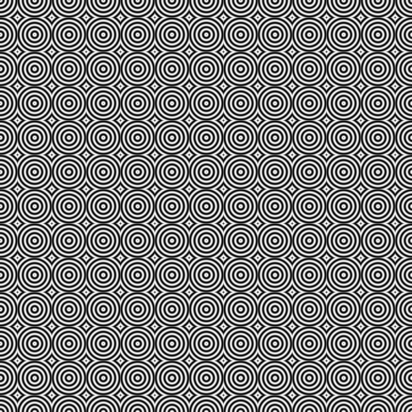
For those who have POV-Ray, a scene file. Image at the end.

// POV-Ray 3.7 
// cmd: +a0.01 +am1  +w500 +h500 +Fpg16 
// ShuheiKawachi.pov
#version 3.7;
global_settings{assumed_gamma 1}
#default{ finish{ambient 0 diffuse 1}} 
camera {
  orthographic
  location <0,0,1> 
  look_at 0 
  right x*image_width/image_height
}

// output range is from [-3, 3]
// POV-Ray clips and folds outside [0,1]
// hence the division by 6 and the addition
// with 0.5 to get te result within [0,1]

// Function from Shuhei Kawachi
// A>0
#declare ShuheiKawachi = function (x,y,z,A,B){
  ((cos(x)*cos(y)+cos((sqrt(A)*x-y)/B)*
  cos((x+sqrt(A)*y)/B)+cos((sqrt(A)*x+y)/B)*
  cos((x-sqrt(A)*y)/B))/6)+0.5
}

#declare PHI = 1.61803399;
plane {
  -z, 0
  texture {
    pigment {
      function{ShuheiKawachi(x,y,z,pi,1.5)}
      scale 0.02
    }
    finish {ambient 1 diffuse 0}
  }
}

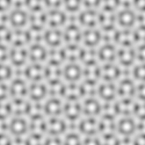
For those who have Python, NumPy and matplotlib:

import numpy as np
from matplotlib import pyplot as plt

PHI = 1.61803399;

#// Shuhei Kawachi
#// A>0, PHI and PI are interesting
def ShuheiKawachi (x,y,A,B):
    f = (np.cos(x)*np.cos(y)+np.cos((np.sqrt(A)*x-y)/B) \
    * np.cos((x+np.sqrt(A)*y)/B)+np.cos((np.sqrt(A)*x+y)/B) \
    * np.cos((x-np.sqrt(A)*y)/B))/3 #division by 3 to bring it in the [-1,1] range
    return f
    
func3d_v = np.vectorize(ShuheiKawachi)

x_interval = (-20, 20)
y_interval = (-20, 20)
x_points = np.linspace(x_interval[0], x_interval[1], 100)
y_points = np.linspace(y_interval[0], y_interval[1], 100)
X, Y = np.meshgrid(x_points, y_points)

Z = func3d_v(X, Y, np.pi, 1.5)

plt.figure(figsize=(5,5))
ax = plt.axes(projection='3d')
ax.plot_surface(X, Y, Z, rstride=1, cstride=1, cmap='gray')
ax.set(xlabel="x", ylabel="y", zlabel="f(x, y)", title="FuncFun")
ax.set_zlim(-3.01, 3.01)

plt.show()
plt.close()

ShuheiKawachi

Just noticed, you can avoid this by passing an audio rate DC

(
{
	Perlin3.ar(
		LFDNoise3.ar(10).range(0, 100), 
		LFDNoise3.ar(10).range(0, 100),
		DC.ar(0) // control rate pitch with 0
	).tanh * 0.5
}.play(s)
)

Thanks for these interesting suggestions !
I had fun especially with the Klein bottle and the border areas of ranges. Therefore I took exponential scaling. Also I always like to experiment with stereo versions. E.g., slightly detuning the Phasor frequency can do this. In this case we can replace the if UGen by Select, as the latter does multichannel expand.

(
Spec.add(\freq_u, [1,2500, \exp]);
Spec.add(\freq_v, [1,2500, \exp]);
Spec.add(\scaleX, [1,250, \exp]);
Spec.add(\scaleY, [1,250, \exp]);
Spec.add(\scaleZ, [1,250, \exp]);
Spec.add(\decorr, [1,1.03, 3]);
)

(
Ndef.new(\pnoise, {
	/*:the Perlin noise is sampled on a klein bottle path.*/
	arg freq_u=100, freq_v=100, decorr = 1.01, scaleX=10, scaleY=10, scaleZ=10, amp = 0.5;
	var r, u, v, x, y, z, grey;
	//klein bottle
	//u -> [0,2*pi];
	//v -> [0,2*pi];
	freq_u = freq_u.lag(0.5);
	freq_v = freq_v.lag(0.5);
	scaleX = scaleX.lag(0.1);
	scaleY = scaleY.lag(0.1);
	scaleZ = scaleZ.lag(0.1);
	
	u = Phasor.ar(0, freq_u * [1, decorr]/SampleRate.ir, start: 0, end: 2*pi);
	v = Phasor.ar(0, freq_v * [decorr, 1]/SampleRate.ir, start: 0, end: 2*pi);
	r = 4*(1-cos(u)/2);
	x = Select.ar(u <= pi, [
		(6*cos(u)*(1+sin(u))+(r*cos(u)*cos(v))),
		(6*cos(u)*(1+sin(u))+(r*cos(v+pi)))
	]);
	y = Select.ar(u <= pi, [
		(16*sin(u)+(r*sin(u)*cos(v))),
		(16*sin(u))
	]);
	z = r*sin(v);
	grey = Perlin3.ar(x/scaleX, y/scaleY, z/scaleZ);
	Out.ar(0, grey * amp);
}).gui;
)

Ndef(\pnoise).clear;

The DC(0) is perfect.
I like the stereo Klein bottle a lot.
It’s about time for me to investigate all the Ugens.
One last ‘scanner’ function. The Supertoroid, a shape shifting torus.

// https://en.wikipedia.org/wiki/Supertoroid

(
Spec.add(\rMajor, [1,25]);
Spec.add(\rMinor, [1,10]);
Spec.add(\tMajor, [0.25,2.5]);
Spec.add(\sMinor, [0.25,2.5]);
Spec.add(\freq_u, [1,250]);
Spec.add(\freq_v, [1,250]);
Spec.add(\scaleX, [0,5]);
Spec.add(\scaleY, [0,5]);
Spec.add(\scaleZ, [0,5]);
)

(
Ndef.new(\pnoise, {
	/*:the Perlin noise is sampled on a supertoroid 3d path with
	given major and minor radius. The shape is controled wit tMajor and sMinor.
	*/
	arg rMajor = 1, rMinor = 0.25
	,tMajor = 1, sMinor = 0.5
	,freq_u=100, freq_v=100
	,scaleX=1, scaleY=1, scaleZ=1
	;
	var u, v, x, y, z, grey;
	//parametric supertoroid
	//u -> [  0   , 2*pi];
	//v -> [  0   , 2*pi];
	u = Phasor.ar(0, freq_u/SampleRate.ir, start: 0, end: 2*pi);
	v = Phasor.ar(0, freq_v/SampleRate.ir, start: 0, end: 2*pi);
	x = cos(u).sign*pow(abs(cos(u)),tMajor)*(rMajor+rMinor*cos(v).sign*pow(abs(cos(v)),sMinor));
	y = sin(u).sign*pow(abs(sin(u)),tMajor)*(rMajor+rMinor*cos(v).sign*pow(abs(cos(v)),sMinor));
	z = rMinor*sin(v).sign*pow(abs(sin(v)),sMinor);
	grey = Perlin3.ar(x/scaleX, y/scaleY, z/scaleZ);
	Out.ar(0, grey!2);
}).gui;
)
Ndef(\pnoise).clear;

Added a second ‘scanning’ circle, more parameters is more fun.


(
Spec.add(\circlefreqC, [0.1,500]);
Spec.add(\radiusC, [1,200]);
Spec.add(\circlefreqD, [1,1200]);
Spec.add(\radiusD, [1,200]);
Spec.add(\centreX, [-50,50]);
Spec.add(\centreY, [-50,50]);
Spec.add(\a, [1,10]);
Spec.add(\b, [0,5]);
)


(
~circ = {
	arg centreX, centreY, radius, circlefreq;
    x = centreX + (radius * SinOsc.ar(circlefreq));
	y = centreY + (radius * SinOsc.ar(circlefreq, pi/2));
	[x,y];
}
)

(
~shuheiKawachi = {
	arg x, y, a, b;
	((cos(x) * cos(y))
	+ (cos((sqrt(a) * x - y) / b)
		* cos((x + (sqrt(a) * y) ) / b))
	+ (cos(( sqrt(a) * x + y) /b)
			* cos((x - (sqrt(a) * y)) / b))) / 3;
};
)

(
Ndef.new(\funfunc, {
	arg radiusC = 40
	, circlefreqC = 10 // circle c drives, moves, the centre point of cirle d.
	, radiusD = 5
	, circlefreqD = 10 // circle d collects the data from the function.
	, centreX=0, centreY=0 
	, a=pi, b=1.5
	;
	var x, y, z, grey;
	var controllcircle = ~circ.(centreX, centreY, radiusC, circlefreqC);
	var datacircle = ~circ.(controllcircle[0], controllcircle[1], radiusD, circlefreqD);
	grey = ~shuheiKawachi.(datacircle[0]/10, datacircle[1]/10, a, b);
	Out.ar(0, grey!2);
}).gui;
)
Ndef(\funfunc).clear;