Frequency instead of phase

thats the first derivation, so far so good:

dphase = 6pi.neg * (1-t).squared;

but whats the nudge? @bovil43810

dphase = dphase / (pi/2 + 0.065); // nudge

That was just me noticing the waveform drifting over time, which I thought could be fixed by multiplying the phase by some symbolic constant. The 0.065 was just based on messing around trying to find such a constant, which didn’t really work obviously. It probably sounds like a stupid way to go about figuring out things like this (which it is, I know) but I’ve been able to solve some problems using this brute force approach, sometimes using RIES or other inverse symbolic lookup tools. Apologies for just kind of dumping that code on you without any further explanation.

What’s the reasoning behind using that exact function ((1-phase)**3 * 2pi) instead of just generating a pitch envelope using Env to get a sine chirp? How did you arrive at it? It’s not in the pulsar chapter in Microsound. If you can’t get an exact number of cycles within the formant period by finding an analytic solution (moving from PM to FM), you can just use a “softer” window than rectangular (e.g. expodec) and won’t get any discontinuities.

It’s not clear to me exactly what kind of result you’re looking for here, especially where FM comes into play. Are you simply trying to do pulsar synthesis with sine chirp pulsarets? Chirps (or chirplets, in this case) obviously already require frequency modulation (a downward or upward pitch sweep). What I’m getting at is: I don’t think what you’re trying to achieve is necessarily impossible because the PM to FM conversion you originally asked about is difficult to figure out analytically, because there may very well be other ways of achieving the same thing that don’t require that sort of derivation, but it’s hard to help you if we don’t know what you’re actually trying to do. Maybe @nathan can help us out here, since they mentioned using downward sine chirps as pulsarets in their blog post, but didn’t include any code examples for that pulsaret type.

thanks for explaining the nudge.
i think for that reason you need to take in account the phase reset.

the formula ((1-phase)**3 * 2pi) comes from @nathan i didnt wanted to bother him any more with all my questions and made it public in the forum. its discribed in his “moisture bass” blog post: Moisture Bass | Nathan Ho
I also thought that the question is more a general one about FM and PM and not so specific about the curved downward sweep. so maybe others would also be interested in the discussion.

the frequency modulation doesnt necessarily come into play there.
i just want to be flexibile enough when writing SynthDefs.
I dont always want to use the chirp and i dont always want to use FM when using patterns to control the instrument.
But both of these things need a different setup at the moment which makes it not possible to interpolate between different timbres.
At the moment i have about 10 SynthDefs which all do some kind of pulsar synthesis. They are similar but not identical. With all of them i was able to create “sound objects” i like. To then compose “timbral evolutions” of these sound objects the different timbres need to be able within the same SynthDef. Thats just my way of doing things in relation to composition.
So i would like to merge some of those concepts which is harder then it seemed to have just one or two SynthDefs in the end.

ive already tried out to use a freq envelope function with a downward sweep scaled to the pulsaret duration or buffered signals for FM driven by the phase. thats cool but you dont get there.

in terms of the envelope generator as far as i understand it:
i think EnvGen would not work here when you modulate freq and formantFreq. you need a stateless envelope function which is driven by the phase.
Therefore i have been trying out IEnvGen. whichs works but is not modulateble which makes it very unflexible.
Ive also tried out buffers which have different problems when switching them and using audio triggers. (BufRd only changes at control rate).

EDIT:
im sorry if have been unprecise. i think one thing about asking questions is that you dont know all the details which are necessary to solve the task. so my initial post was my attempt to formulate the question in the most condensed way i was able to. thanks for taking some time :slight_smile:

I haven’t taken the time to read through and fully understand this thread, so sorry if I’m missing something basic, but I can explain my chirp formula.

I start with a periodic signal, called pulsaretPhase in my blog post, that is 0 at the beginning of the pulsaret, 1 at the end, and continues linearly increasing during the silence at the same rate before resetting to 0 at the start of the next pulsaret. It looks like a saw wave signal, so I used an LFSaw to generate it. You can also use Sweep/Impulse if you want.

To get a single sine wave cycle for your pulsaret, the formula is (pulsaretPhase * 2pi).sin. To get multiple sine wave cycles, use (pulsaretPhase * numSineCycles * 2pi).sin.

Now, to get a chirp, I use a nonlinear function of pulsaretPhase as an input to the sin function. The nonlinear function I decided to use was x ** 3, which curves the range [0, 1] so that it starts off slow, speeds up and rapidly approaches 1. However, a chirp starts off fast and slows down, so we use the time reversal of this instead: (1 - x) ** 3. The resulting pulsaret function is therefore ((1 - pulsaretPhase) ** 3 * numSineCycles * 2pi).sin. This is what I used in the second audio example in my blog post.

I haven’t tried combining FM or PM with pulsar synthesis, so I don’t know anything about that.

1 Like

I tried to write down the derivation @dietcv asked for in the original post to see whether I made any mistakes. Bascially, it boils down to finding the instantaneous frequency given the instantaneous phase, like hjh said.

We start by writing out the phase modulation formulation:

y(t) = sin((1 - phase) ** 3 * 2pi), where phase = t * formantFreq
y(t) = sin((1 - (t * formantFreq)) ** 3 * 2pi)

We denote the argument of the sine, which is the instantaneous phase, as phi(t):

y(t) = sin(phi(t)) where phi(t) = (1 - (t * formantFreq)) ** 3 * 2pi)

Then, the instaneous frequency, which is the derivative of the phase and denoted omega(t) = phi'(t) = d/dt phi(t), can be calculated as follows:

phi'(t)  = d/dt (1 - (t * formantFreq)) ** 3 * 2pi)
phi'(t) = 2pi * d/dt (1 - (t * formantFreq)) ** 3)                              // take out constant
phi'(t) = 2pi * 3 * ((1 - (t * formantFreq)) ** 2) d/dt (1 - (t * formantFreq)) // apply chain rule: d/dt (t**a) = a * ( t**(a-1))
phi'(t) = 2pi * 3 * ((1 - (t * formantFreq)) ** 2) * (-formantFreq)             // d/dt (1 - (a*t)) = -a

which simplifies to:

omega(t) = phi'(t) = -6pi * formantFreq * ((1 - (t * formantFreq)) ** 2)

However, that gives us the instantaneous angular frequency (in rad/s), which we still need to convert to the instantaneous ordinary frequency (in Hz):

f(t) = omega(t) / 2pi = -3 * formantFreq * ((1 - (t * formantFreq)) ** 2)

Translated to code:

(
{
	var t, phi, f, fm, pm;
	var freq = 100;
	var formantFreq = 400;	
	
	t = Sweep.ar;
	phi = (1 - (t * formantFreq)) ** 3 * 2pi;
	f = 3.neg * formantFreq * (1 - (t * formantFreq)).squared;

	pm = SinOsc.ar(0, phi.mod(2pi));
	fm = SinOsc.ar(f);

	[pm, fm]
}.plot(0.01).superpose_(true).plotColor_([Color.red, Color.green]);
)

Unfortunately, there still is a visible and audible discrepancy in the result which I can’t explain, but the conversion method itself is sound.

thanks alot for the detailed explanation :slight_smile:

When you add the rectangular window like in my initial example, you can see that the phase reset is still a problem, every pulsaret is different.
When you additionally change freq and FormantFreq you see that the difference between the two formulas is even bigger.

(
{
	var t, phi, f, fm, pm;
	var freq = 100;
	var formantFreq = 800;
	var trig = Impulse.ar(freq);

	t = Sweep.ar(trig);
	phi = (1 - (t * formantFreq)) ** 3 * 2pi;
	f = 3.neg * formantFreq * (1 - (t * formantFreq)).squared;

	pm = SinOsc.ar(0, phi.mod(2pi));
	fm = SinOsc.ar(f);

	pm = pm * (t * formantFreq < 1.00);
	fm = fm * (t * formantFreq < 1.00);

	[pm, fm]
}.plot(0.02).superpose_(true).plotColor_([Color.red, Color.green]);
)

ive experimented a bit more with fm and pm for pulsar synthesis. still trying to find out how to make these two expressions identical, to be able to get rid of the curved phase and have a more versatile fm expression.
what kind of FM modulator do you need for having an ordinary fm approach like this:

fm_phase = Sweep.ar(trig, grainFreq * (1 + (fmod * index)));

and be able to get the same result? thanks

(
{
	var tFreq = 100;
	var grainFreq = 400;
	var trig = Impulse.ar(tFreq);
	
	var pm_phase = Sweep.ar(trig, grainFreq);
	var fm_phase = Sweep.ar(trig, grainFreq * (1 + (LFSaw.ar(grainFreq, 1) * \index.kr(1))));

	var pm = sin((1 - pm_phase) ** 3 * 2pi);
	var fm = sin(fm_phase * 2pi);

	pm = pm * (pm_phase < 1.00);
	fm = fm * (fm_phase < 1.00);

	[pm, fm]
}.plot(0.02);
)

when i look at the phases there is this little bump in the end for FM, whats causing this? Its not so much about the plot, but they are also sounding differently and i would like to get rid of (1 - fm_phase) and have fm_phase instead.

(
{
	var tFreq = 100;
	var grainFreq = 400;
	var trig = Impulse.ar(tFreq);

	var pm_phase = Sweep.ar(trig, grainFreq);
	var fm_phase = Sweep.ar(trig, grainFreq * (1 + LFSaw.ar(grainFreq, 1).neg));
	
	var pm_grainWindow = pm_phase < 1;
	var fm_grainWindow = fm_phase < 1;
	
	pm_phase = (1 - pm_phase) ** 3;
	fm_phase = (1 - fm_phase);
	
	pm_phase = pm_phase * pm_grainWindow;
	fm_phase = fm_phase * fm_grainWindow;
	
	[pm_phase, fm_phase];
}.plot(0.005);
)

if its necessary i could also think of using PlayBuf as a modulator for FM with a buffered single cycle signal to get the desired result.

made some further adjustments, still not sure how to get the curved phase with the FM approach.

(
{
	var tFreq = 400;
	var grainFreq = 800;
	var trig = Impulse.ar(tFreq);
	var overlap = 2;

	var pm_phase = Sweep.ar(trig, grainFreq);

	//var fmod = (grainFreq / tFreq) - Sweep.ar(trig, grainFreq);
	//var fm_phase = Sweep.ar(trig, grainFreq * fmod);

	var fm_phase = Sweep.ar(trig, grainFreq * (1 + SinOsc.ar(tFreq, 0.5pi)));

	var pm_grainWindow = pm_phase / overlap < 1;
	var fm_grainWindow = fm_phase / overlap < 1;

	pm_phase = (1 - pm_phase) ** 3;
	fm_phase = (1 - fm_phase);

	pm_phase = pm_phase * pm_grainWindow;
	fm_phase = fm_phase * fm_grainWindow;

	[pm_phase, fm_phase];
}.plot(0.005);
)

Just throwing this into the conversation, Bill Schottstaedt offers a very nice overview in his An Introduction To FM. In his introduction, Schottstaedt states “… there is no essential difference between frequency and phase modulation.”

Schottstaedt presents a number of implementations (in CLM), along with analysis and discussion.

1 Like

thanks for the link. this is a real headscratcher to me:

(
{	
	var tFreq = 400;
	var trig = Impulse.ar(tFreq);
	var grainFreq = 800;
	var overlap = 1;
	
	var phase = Sweep.ar(trig, grainFreq);
	
	var fmod = 3.neg * (1 - Sweep.ar(trig, grainFreq)).squared;
	var fm_phase = Sweep.ar(trig, grainFreq * fmod);
	
	var grainWindow = phase / overlap < 1;
	
	var pm_sig = sin((1 - phase) ** 3 * 2pi);
	var fm_sig = sin(fm_phase * 2pi);
	
	pm_sig = pm_sig * grainWindow;
	fm_sig = fm_sig * grainWindow;

	[pm_sig, fm_sig];
}.plot(0.005);
)

(
{
	var tFreq = 100;
	var trig = Impulse.ar(tFreq);
	var grainFreq = 400;
	var overlap = MouseY.kr(1, 2);

	var phase = Sweep.ar(trig, grainFreq);

	var fmod = 3.neg * (1 - (Sweep.ar(trig, grainFreq))).squared;
	var fm_phase = Sweep.ar(trig, grainFreq * fmod);

	var pm_grainWindow = phase / overlap < 1;
	var fm_grainWindow = fm_phase / overlap < 1;

	var pm_sig = sin((1 - phase) ** 3 * 2pi);
	var fm_sig = sin(fm_phase * 2pi);

	var sig;
	
	pm_sig = pm_sig * pm_grainWindow;
	fm_sig = fm_sig * pm_grainWindow;

	sig = LinXFade2.ar(pm_sig, fm_sig, MouseX.kr(-1, 1));
	sig !2 * 0.1;
	
}.scope;
)

I still think my earlier suggestion is the best one worth not forgetting.

If you want the solution to be completely exact, you need somebody who is good in calculus. Otherwise you’re just stabbing randomly in the dark, and you will not accidentally find the solution that way.

Schottstaedt states “… there is no essential difference between frequency and phase modulation.”

Yes, because phase is the integral of frequency (and frequency is the derivative of phase). In classic FM, when you adding a sinusoid to a constant frequency, then the phase is the integral of these two terms.

  • a = integral of constant frequency = f * t – a line (ramp).
  • b = integral of sinusoid = phase-shifted sinusoid. (Integral of cosine = sine.)
  • FM’ed phase = a + b

And you can go the other way (PM synthesis). If you start with a linear ramp for phase, and add a sinusoid, the effect on frequency is:

  • a = derivative of linear ramp = constant frequency.
  • b = derivative of sinusoid = phase-shifted sinusoid.
  • Add those together, and it’s FM.

The catch is – and what often happens in FM – is that the modulator might have its own DC offset. (This happens easily, say, in a three-operator chain: A → B → C. A → B is likely to have DC offset.) Then the frequency is a (constant frequency) + b (modulator without DC offset) + c (modulator’s DC offset, constant value) = sum of two constant values (shifts the whole frequency!) + modulator b = not the frequency you started with.

In this case, you might think everything is keying off the same basic frequency, but you don’t get the nice clean tone color.

But PM, in the same situation, doesn’t have this effect, because the DC offset in the modulator only phase-shifts the wave in time, but does not skew frequency. This is why (I think) most FM synthesizers are really PM synthesizers.

@dietcv, your fmod does have a negative DC offset, skewing frequency downward. This might be the reason why it isn’t getting all the way back to 0 by the end of the grain. If I’m right, then your FM approach would have to control for DC offset. (If you’re not sure how to do that… again… take a mathematician out for a beer – or accept that PM handles DC offset better than FM and just use PM.)

hjh

thanks for your further explanations.

i think one solution then would be to stay with PM but exchange (1 - phase) ** 3 for a more general PM expression where pmod could either be an Oscillator or Playbuf.

(
{
	var tFreq = 100;
	var trig = Impulse.ar(tFreq);
	var grainFreq = 400;

	var phase = Sweep.ar(trig, grainFreq);
	
	//var pmod = ???
	//var sig = sin(phase * (1 + (pmod * index)) * 2pi);
	var sig = sin((1 - phase) ** 3 * 2pi);

	var grainWindow = phase < 1;

	sig = sig * grainWindow;

	sig;

}.plot(0.02);
)

Does somebody know how this would look like for this specific case?

Is this what you were looking for? Phase modulation with a waveform read from a buffer.

What I have not been able to figure out so far is how this would work if the carrier was also a BufRd, rather than sin( (phase * 2pi)). I’d be grateful for suggestions.

b=Buffer.loadCollection(s, Signal.sineFill(2048, [1,00], 0!2))

(
{
	arg phase_buf = 0, form = 1, mod_depth = 1;


	var tFreq = 100;
	var trig = Impulse.ar(tFreq);

	var phase = Sweep.ar(trig, tFreq*form.max(1));

	var phase_mod = BufRd.ar(1, phase_buf, phase*BufFrames.kr(phase_buf), 1, 2);

	var sig = sin( (phase * 2pi) + (phase_mod * mod_depth).mod(2pi) );
	
	var grainWindow = phase < 1;

	sig = sig * grainWindow;

	sig

}.plot(0.02)
)

thanks alot for your help :slight_smile:

in this thread are some hints for such an implementation, which i cannot make any sense of in my case.
The Sweep.ar rate cant be multiplied by BufFrames.kr(b) * bufRateScale.ir(b) because its phase is also used for the grain window (this is fixed) and phi is not a BufRd but a SinOsc.
Here is my extraction of the pm example from the thread:

(
{
	var carr = 100;
	var mod = 200;
	var index = 2;

	var bufFrames = BufFrames.ir(b);
	var phase = Sweep.ar(0, carr * bufFrames * BufRateScale.ir(b));
	var phi = ((1 - SinOsc.ar(mod, pi/2)) * index).mod(2pi);

	var sig = BufRd.ar(1, b, (phase + (phi * bufFrames * BufRateScale.ir(b) / 2pi)).mod(bufFrames));

	sig;
	
}.plot(0.02)
)

however none of these examples does give me the desired end result. the phase modulator isnt a plain sine wave.

(
{	
	var tFreq = 100;
	var trig = Impulse.ar(tFreq);
	var grainFreq = 400;
	
	var phase = Sweep.ar(trig, grainFreq);
	
	var grainWindow = phase < 1;
	
	var sig = sin((1 - phase) ** 3 * 2pi);
	
	sig = sig * grainWindow;

	sig;
}.plot(0.005);
)

Thanks @dietcv for pointing me to that other thread and for suggesting a way to adapt it.

This is still a little messy, but it works:

b=Buffer.loadCollection(s, Signal.sineFill(2048, {rrand(0.0,1.0)}!3, 0!3))

(
{
	var carr = 100;
	var mod = 10;
	var index = 0.2;

	var bufFrames = BufFrames.kr(b);
	var phase = Sweep.ar(0, carr * bufFrames * BufRateScale.kr(b));

	var phi = (( 1 - BufRd.ar(1, b, (mod* phase + (0.25 * bufFrames * BufRateScale.kr(b))), 1, 2)) * index ).mod(2pi);

	var sig = BufRd.ar(1, b, (phase + (phi * bufFrames * BufRateScale.kr(b) / 2pi)).mod(bufFrames));

	sig;

}.plot(0.02)
)

Sorry this is still not the solution you are looking for!

ok i think i got it!!!

this is an ordinary PM implementation, just with an added window and a flipped phase for better comparision:

// ordinary PM

(
{
	var freq = 400;
	var mod = SinOsc.ar(freq * \mRatio.kr(1));
	var sig = SinOsc.ar(freq * \cRatio.kr(1), (mod * \index.kr(5)).wrap(0, 4pi));
	sig.neg * (Sweep.ar(0, freq) < 1);
}.plot(0.005);
)

this BufRd pulsar implementation leads to the same result:

(
~freqBuf = Buffer.loadCollection(s, Signal.sineFill(2048, [1,0], 0!2));
~sndBuf = Buffer.loadCollection(s, Signal.sineFill(4096, [1,0], 0!2));
)

// pulsar BufRd PM with two sinusoids:

(
{
	var tFreq = \tFreq.kr(100);
	var trig = Impulse.ar(tFreq);
	var grainFreq = \freq.kr(400);
	var phase = Sweep.ar(trig, grainFreq);

	var phi = BufRd.ar(
		numChannels: 1,
		bufnum: ~freqBuf,
		phase: phase * BufFrames.kr(~freqBuf),
		loop: 0,
		interpolation: 4
	);

	var sig = BufRd.ar(
		numChannels: 1,
		bufnum: ~sndBuf,
		phase: 1 - (phase + ((phi * \index.kr(5)) / 2pi)) * BufFrames.kr(~sndBuf),
		loop: 1,
		interpolation: 4
	);

	sig * (phase < 1);

}.plot(0.005);
)

when instead using a welch window as the modulator and decreasing the modulation index from 5 to 2 you get the curved phase signal:

(
var welch = Env([0, 1, 0], [0.5, 0.5], \wel).discretize(4096);
~freqBuf = Buffer.sendCollection(s, welch, 1);
~sndBuf = Buffer.loadCollection(s, Signal.sineFill(4096, [1,0], 0!2));
)

// pulsar BufRd PM with welch window as a modulator

(
{
	var tFreq = \tFreq.kr(100);
	var trig = Impulse.ar(tFreq);
	var grainFreq = \freq.kr(400);
	var phase = Sweep.ar(trig, grainFreq);

	var phi = BufRd.ar(
		numChannels: 1,
		bufnum: ~freqBuf,
		phase: phase * BufFrames.kr(~freqBuf),
		loop: 0,
		interpolation: 4
	);

	var sig = BufRd.ar(
		numChannels: 1,
		bufnum: ~sndBuf,
		phase: 1 - (phase + ((phi * \index.kr(2)) / 2pi)) * BufFrames.kr(~sndBuf),
		loop: 1,
		interpolation: 4
	);

	sig * (phase < 1);

}.plot(0.005);
)

EDIT: i think the use of the welch window shows really nicely how frequency and phase are relatives of each other. Im wondering if i could use a ramp instead of a welch window when changing the interface.
thinking in terms of frequencies is a bit more straighforward then thinking of integrated frequency changes.
But i think the ordinary SinOsc as a modulator would not work anymore when changing the interface.

EDIT: using a curved ramp as the phase modulator and multiplying phi with the phase again does lead to something similiar, but then the SinOsc implementation doesnt work anymore, so ive introduced an index window:

(
var ramp = Env([1, 0], [1], [3.0]).discretize(4096);
~freqBuf = Buffer.sendCollection(s, ramp, 1);
~sndBuf = Buffer.loadCollection(s, Signal.sineFill(4096, [1,0], 0!2));
)

(
var statelessWindow = { |levels, times, curve, phase|
	var x = 0;
	var window = times.size.collect{ |i|
		var x2 = x + times[i];
		var result = (phase >= x) * (phase < x2) * phase.lincurve(x, x2, levels[i], levels[i+1], curve[i]);
		x = x2;
		result;
	}.sum;
	window * (phase < 1);
};

{
	var tFreq = \tFreq.kr(100);
	var trig = Impulse.ar(tFreq);
	var grainFreq = \freq.kr(400);
	var phase = Sweep.ar(trig, grainFreq);

	var phi = BufRd.ar(
		numChannels: 1,
		bufnum: ~freqBuf,
		phase: phase * BufFrames.kr(~freqBuf),
		loop: 0,
		interpolation: 4
	);

	var indexWindow = statelessWindow.(
		levels: [0, 1],
		times: [1],
		curve: [-8.0],
		phase: phase
	);
	var index = \index.kr(0) + indexWindow.linlin(0, 1, 0, \indexModAmount.kr(2));

	var sig = BufRd.ar(
		numChannels: 1,
		bufnum: ~sndBuf,
		phase: 1 - (phase + ((phi * index) / 2pi)) * BufFrames.kr(~sndBuf),
		loop: 1,
		interpolation: 4
	);

	sig * (phase < 1);

}.plot(0.005);
)

any suggestions?

The welch window created by EnvGen is actually a half-sine window:

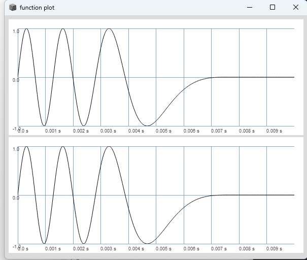
if you take the derivative of the half sine window which is a half cosine window and add ((grainFreq / overlap) * SampleDur.ir) to fmod, PM and FM are pretty much identical:

(
{
	var tFreq = 100;
	var trig = Impulse.ar(tFreq);
	var grainFreq = 400;
	var overlap = \overlap.kr(3).clip(0, grainFreq / tFreq);

	var phase = Sweep.ar(trig, grainFreq);
	var windowPhase = phase / overlap;
	var rectWindow = windowPhase < 1;

	var fmod = cos(windowPhase * pi) + ((grainFreq / overlap) * SampleDur.ir);
	var fm_phase = Sweep.ar(trig, grainFreq * (1 + (fmod * \index.kr(1))));

	var pmod = sin(windowPhase * pi);
	var pm_phase = phase + ((pmod * overlap) / pi);

	var pm_sig = sin(pm_phase * 2pi);
	var fm_sig = sin(fm_phase * 2pi);

	[pm_sig * rectWindow, fm_sig * rectWindow];

}.plot(0.01);
)

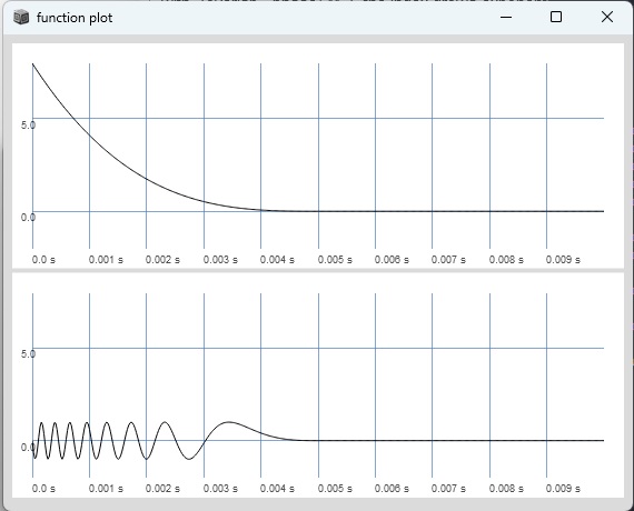
(1 - phase) ** 3 is quite similiar for overlap == 1. If you increase overlap and exchange (1 - phase) ** 3 with (overlap - phase) ** 3 the index grows exponentially if you change overlap, with the half cosine window for FM or the half sine window for PM the index grows linearly when you change overlap.

(
{
	var tFreq = 100;
	var trig = Impulse.ar(tFreq);
	var grainFreq = 400;
	var phase = Sweep.ar(trig, grainFreq);
	var overlap = \overlap.kr(2).clip(0, grainFreq / tFreq);

	var windowPhase = phase / overlap;
	var rectWindow = windowPhase < 1;

	var pulsaretPhase = (overlap - phase) ** 3;
	
	var sig = sin(pulsaretPhase * 2pi);
	
	[pulsaretPhase * rectWindow, sig * rectWindow];

}.plot(0.01);
)

rgaighi