This is a first sketch of the first part for the helpfile of the grain utils. You can find an A / B example in section 4c. The second part will be implemented as well.
TITLE::Event Scheduling
summary::sub-sample accurate event scheduling
categories::UGens>Triggers, Libraries>Timing, Streams-Patterns-Events>Timing
related::Classes/Phasor, Classes/Impulse, Classes/GrainBuf
DESCRIPTION::
Sub-sample accurate phasor-based scheduling provides precise timing control for audio events by using continuous, linear ramps instead of discrete triggers.
This approach offers significant advantages over trigger-based scheduling by providing continuous time information and sub-sample timing accuracy.
Unlike trigger-based systems that only provide timing information at discrete moments, phasor-based scheduling gives you continuous access to:
list::
## Elapsed time since the last event
## Remaining time until the next event
## Fractional sample positions for precise timing
::
This technique is particularly valuable for any application requiring high-timing accuracy beyond the sample rate resolution, for example granular synthesis.
SECTION::1) Continuous Linear Ramps as a Source of Time
subsection::1a) The Scheduling Phasor
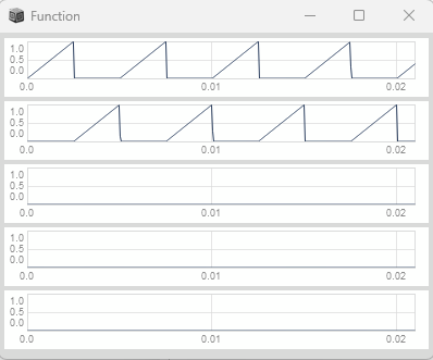
The source of time (our clock) is a Phasor creating continuous, linear ramps between 0 and 1.
The rate parameter of the Phasor determines the density of events - how frequently the phasor completes each cycle and wraps back around,
with each wrap representing a timing event.
list::
## strong::Continuous:: continuously wrapping between 0 and 1 (no phase reset) - This preserves the fractional sample position where the wrap occurs, which contains the sub-sample timing information
## strong::Linear:: Constant rate of change per sample for every cycle, providing predictable timing relationships
## strong::Normalized:: Normalized range between 0 and 1 that simplifies calculations
::
code::
(
{
var rate = 1000; // 1000 events per second
Phasor.ar(DC.ar(0), rate * SampleDur.ir);
}.plot(0.0021).plotMode_(\plines); // Observe the continuous, linear ramps between 0 and 1
)
::
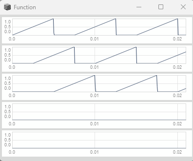
subsection::1b) Deriving Triggers from a Scheduling Phasor
To convert the continuous ramp into discrete timing events, we need to derive a trigger from our scheduling phasor at the moment it wraps around.
subsubsection::Magnitude Delta Method
The simplest method of deriving a trigger from a phasor's wrap, is to calculate its slope (rate of change per sample)
and compare that with a threshold. When the phasor wraps from 1 to 0, the absolute delta becomes large (approximately 1) and we output a trigger.
code::
(
var rampToTrig = { |phase|
var history = Delay1.ar(phase); // Previous sample value
var delta = phase - history; // Rate of change per sample
delta.abs > 0.5; // Trigger when absolute delta exceeds threshold
};
{
var phase, trig;
phase = Phasor.ar(DC.ar(0), 1000 * SampleDur.ir);
trig = rampToTrig.(phase);
[phase, trig];
}.plot(0.0021).plotMode_(\plines);
)
::
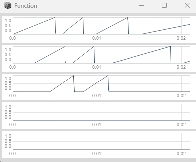
subsubsection::Proportional Change Method (Recommended)
You may have noticed on the prior plot that we don't get an initial trigger from the magnitude delta method.
We additionally don't get a trigger if we would manually reset our scheduling phasor in the first half of its duty cycle.
But we can handle both of these limitations with the proportional change method.
Instead of comparing the raw delta with a threshold, we calculate the proportional change by dividing the delta by the sum of the current and previous sample values,
and then compare this absolute proportional change with our threshold to detect a significant change.
To make sure we only get triggers on false-to-true transitions (extreme inputs do not cause double triggers), we wrap our trigger into link::Classes/Trig1::.
code::
(
var rampToTrig = { |phase|
var history = Delay1.ar(phase);
var delta = phase - history; // Rate of change
var sum = phase + history; // Signal magnitude reference
var trig = (delta / sum).abs > 0.5; // Proportional change detection
Trig1.ar(trig, SampleDur.ir); // Ensure triggers on false-to-true transitions only
};
{
var phase, trig;
phase = Phasor.ar(DC.ar(0), 1000 * SampleDur.ir);
trig = rampToTrig.(phase);
[phase, trig];
}.plot(0.0021).plotMode_(\plines);
)
::
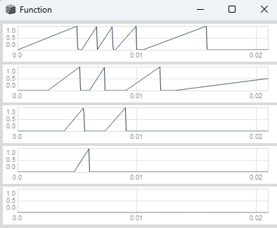
subsection::1c) Deriving Slopes from a Scheduling Phasor
Deriving the slope of the phasor gives us its rate of change per sample (normalized frequency).
At the phasor's wrap we get a discontinuity in slope, which we used earlier for our trigger detection.
Our derived slope should be a continuous value for each phasor's cycle without any discontinuities.
To achieve that we can wrap the derived slope between -0.5 and 0.5 (nyquist frequency).
The slope multiplied by the sample rate gives us frequency in Hz.
code::
(
var rampToSlope = { |phase|
var history = Delay1.ar(phase);
var delta = phase - history;
delta.wrap(-0.5, 0.5); // Handle discontinuity at the phasor's wrap
};
{
var rate, phase, slope;
rate = 1000;
phase = Phasor.ar(DC.ar(0), rate * SampleDur.ir);
slope = rampToSlope.(phase);
[phase, slope * SampleRate.ir / 1000]; // Scale slope for visualization purposes
}.plot(0.0021).plotMode_(\plines);
)
::
SECTION::2) Accumulating vs Integrating Ramps from a Scheduling Phasor
The crucial distinction between these two approaches is their handling of frequency modulation:
list::
## strong::Accumulation:: counts samples and scales running total with slope. The slope has to be sampled and held for each cycle - no frequency modulation possible
## strong::Integration:: adds up slope values for every sample - supports frequency modulation
::
subsection::2a) Using Duty for Accumulation
We first derive the slope and triggers from our scheduling phasor.
Then we count samples with Duty and scale the running total of the accumulator by the derived slope and reset it by the derived trigger.
code::
(
var rampToTrig = { |phase|
var history = Delay1.ar(phase);
var delta = phase - history;
var sum = phase + history;
var trig = (delta / sum).abs > 0.5;
Trig1.ar(trig, SampleDur.ir);
};
var rampToSlope = { |phase|
var history = Delay1.ar(phase);
var delta = phase - history;
delta.wrap(-0.5, 0.5);
};
var accum = { |trig|
var hasTriggered = PulseCount.ar(trig) > 0;
Duty.ar(SampleDur.ir, trig, Dseries(0, 1)) * hasTriggered;
};
{
var phase, trig, slope, accumulator, accumulatedRamp;
phase = Phasor.ar(DC.ar(0), 1000 * SampleDur.ir);
trig = rampToTrig.(phase);
slope = rampToSlope.(phase);
accumulator = accum.(trig);
accumulatedRamp = Latch.ar(slope, trig) * accumulator; // Constant slope per cycle
[phase, trig, accumulatedRamp];
}.plot(0.0021).plotMode_(\plines);
)
::
subsection::2b) Using Sweep for Integration
We first derive the slope and triggers from our scheduling phasor.
Then we integrate the derived slope values with Sweep and reset the integrator by the derived trigger.
code::
(
var rampToTrig = { |phase|
var history = Delay1.ar(phase);
var delta = phase - history;
var sum = phase + history;
var trig = (delta / sum).abs > 0.5;
Trig1.ar(trig, SampleDur.ir);
};
var rampToSlope = { |phase|
var history = Delay1.ar(phase);
var delta = phase - history;
delta.wrap(-0.5, 0.5);
};
var ramp = { |trig, slope|
var hasTriggered = PulseCount.ar(trig) > 0;
Sweep.ar(trig, slope * SampleRate.ir) * hasTriggered;
};
{
var phase, trig, slope, integratedRamp;
phase = Phasor.ar(DC.ar(0), 1000 * SampleDur.ir);
trig = rampToTrig.(phase);
slope = rampToSlope.(phase);
integratedRamp = ramp.(trig, slope); // Continuous integration
[phase, trig, integratedRamp];
}.plot(0.0021).plotMode_(\plines);
)
::
SECTION::3) Ramp Division
In the prior section we have recreated our initial scheduling phasor by accumulation or integration.
Instead of just recreating our scheduling phasor, we can accumulate or integrate ramps which are subdivisions of our scheduling phasor.
This is similiar to a Clock Divider. However the advantage of ramp division vs clock division is that ramp division is possible
with non-integer ratios and the derived events can be sub-sample accurate (we will look at this more closely in section 4).
subsection::3a) Multiply and Wrap
The simplest way of ramp division is to multiply the phasor by a ratio and wrap the result between 0 and 1.
code::
(
{
var phase, subdividedRamp;
phase = Phasor.ar(DC.ar(0), \rate.kr(100) * SampleDur.ir);
subdividedRamp = (phase * \ratio.kr(4)).wrap(0, 1);
[phase, subdividedRamp];
}.plot(0.021);
)
::
subsection::3b) Accumulation with Triggered Reset
With the simple multiply and wrap approach, we cant ensure that our subvidided ramps stay perfectly in sync with our scheduling phasor.
To make sure our subdivided ramps stay perfectly in sync, we can derive the slope and triggers from our scheduling phasor,
run an accumulator and multiply it by the slope and a ratio, reset it by the derived triggers and wrap it between 0 and 1.
The triggered reset is the only way of keeping the subdivided ramps perfectly in sync with our scheduling phasor. Thats what we are going to use for granulation.
code::
(
var rampToSlope = { |phase|
var history = Delay1.ar(phase);
var delta = phase - history;
delta.wrap(-0.5, 0.5);
};
var rampToTrig = { |phase|
var history = Delay1.ar(phase);
var delta = phase - history;
var sum = phase + history;
var trig = (delta / sum).abs > 0.5;
Trig1.ar(trig, SampleDur.ir);
};
{
var phase, slope, trig, accumulator, subdividedRamp;
phase = Phasor.ar(DC.ar(0), \rate.kr(100) * SampleDur.ir);
slope = rampToSlope.(phase);
trig = rampToTrig.(phase);
accumulator = Duty.ar(SampleDur.ir, trig, Dseries(0, 1));
subdividedRamp = (slope * \ratio.kr(4) * accumulator).wrap(0, 1);
[phase, subdividedRamp];
}.plot(0.021);
)
::
subsection::3c) Accumulation without Triggered Reset
The only way we can accumulate ramps which are slower than our scheduling phasor,
is either to use multichannel expansion which we are going to use for granulation or to simply run an accumulator without a triggered reset.
To make sure our accumulated ramps can be slower, we can derive the slope from our scheduling phasor, run an accumulator and multiply it by the slope
and a ratio and wrap it between 0 and 1. But there is no guarantee that these accumulated ramps will stay in sync with the scheduling phasor.
code::
(
var rampToSlope = { |phase|
var history = Delay1.ar(phase);
var delta = phase - history;
delta.wrap(-0.5, 0.5);
};
{
var phase, slope, accumulator, subdividedRamp;
phase = Phasor.ar(DC.ar(0), \rate.kr(100) * SampleDur.ir);
slope = rampToSlope.(phase);
accumulator = Duty.ar(SampleDur.ir, DC.ar(0), Dseries(0, 1));
subdividedRamp = (slope * \ratio.kr(0.5) * accumulator).wrap(0, 1);
[phase, subdividedRamp];
}.plot(0.021);
)
::
SECTION::4) Sub-Sample Offset Calculation
If we run our scheduling phasor at high trigger rates which are non-integer divisions of our sample rate we get aliasing.
Our scheduling phasor has a fractional value of non-zero at the moment it wraps around (sub-sample offset).
To make sure our accumulated or integrated ramps are sub-sample accurate, we want to calculate the sub-sample offset of our scheduling phasor and add it to
our accumulated or integrated ramps on each triggered phase reset.
For each sample frame where our scheduling phasor wraps around, we can calculate the sub-sample offset with a fractional sample counter
(scheduling phasor divided by its own slope), sample and hold the fractional sample count with the derived trigger
and add the fractional sample count (sub-sample offset) to our accumulated or integrated ramps on each triggered phase reset.
subsection::4a) Sub-Sample Offset Calculation (accumulator with Duty)
code::
(
var rampToTrig = { |phase|
var history = Delay1.ar(phase);
var delta = phase - history;
var sum = phase + history;
var trig = (delta / sum).abs > 0.5;
Trig1.ar(trig, SampleDur.ir);
};
var rampToSlope = { |phase|
var history = Delay1.ar(phase);
var delta = phase - history;
delta.wrap(-0.5, 0.5);
};
var getSubSampleOffset = { |phase, slope, trig|
var sampleCount = phase / slope;
Latch.ar(sampleCount, trig);
};
var accumSubSample = { |trig, subSampleOffset|
var hasTriggered = PulseCount.ar(trig) > 0;
var accum = Duty.ar(SampleDur.ir, trig, Dseries(0, 1)) * hasTriggered;
accum + subSampleOffset;
};
{
var eventPhase, eventTrigger, eventSlope;
var subSampleOffset, accumulator;
var accumulatedRamp;
eventPhase = Phasor.ar(DC.ar(0), 1000 * SampleDur.ir);
eventSlope = rampToSlope.(eventPhase);
eventTrigger = rampToTrig.(eventPhase);
subSampleOffset = getSubSampleOffset.(eventPhase, eventSlope, eventTrigger);
accumulator = accumSubSample.(eventTrigger, subSampleOffset);
accumulatedRamp = eventSlope * accumulator;
[eventPhase, eventTrigger, accumulatedRamp];
}.plot(0.0011).plotMode_(\plines);
)
::
subsection::4b) Sub-Sample Offset Calculation (integrator with Sweep)
code::
(
var rampToTrig = { |phase|
var history = Delay1.ar(phase);
var delta = phase - history;
var sum = phase + history;
var trig = (delta / sum).abs > 0.5;
Trig1.ar(trig, SampleDur.ir);
};
var rampToSlope = { |phase|
var history = Delay1.ar(phase);
var delta = phase - history;
delta.wrap(-0.5, 0.5);
};
var getSubSampleOffset = { |phase, slope, trig|
var sampleCount = phase / slope;
Latch.ar(sampleCount, trig);
};
var integSubSample = { |trig, slope, subSampleOffset|
var hasTriggered = PulseCount.ar(trig) > 0;
var accum = Sweep.ar(trig, slope * SampleRate.ir) * hasTriggered;
accum + (slope * subSampleOffset);
};
{
var eventPhase, eventTrigger, eventSlope;
var subSampleOffset, integratedRamp;
eventPhase = Phasor.ar(DC.ar(0), 1000 * SampleDur.ir);
eventSlope = rampToSlope.(eventPhase);
eventTrigger = rampToTrig.(eventPhase);
subSampleOffset = getSubSampleOffset.(eventPhase, eventSlope, eventTrigger);
integratedRamp = integSubSample.(eventTrigger, eventSlope, subSampleOffset);
[eventPhase, eventTrigger, integratedRamp];
}.plot(0.0011).plotMode_(\plines);
)
::
subsection::4c) sub-sample accurate scheduling vs trigger-based scheduling
You can compare our sub-sample accurate phasor-based scheduling with ordinary trigger-based scheduling with the following examples.
The first example uses our sub-sample accurate phasor-based scheduling, where the other uses trigger-based scheduling.
Running both examples, you will hear and see the difference on the freqscope.
code::
// sub-sample accurate phasor-based scheduling
(
var rampToSlope = { |phase|
var history = Delay1.ar(phase);
var delta = (phase - history);
delta.wrap(-0.5, 0.5);
};
var rampToTrig = { |phase|
var history = Delay1.ar(phase);
var delta = phase - history;
var sum = phase + history;
var trig = (delta / sum).abs > 0.5;
Trig1.ar(trig, SampleDur.ir);
};
var getSubSampleOffset = { |phase, slope, trig|
var sampleCount = phase / slope;
Latch.ar(sampleCount, trig);
};
var accumulatorSubSample = { |trig, subSampleOffset|
var hasTriggered = PulseCount.ar(trig) > 0;
var accum = Duty.ar(SampleDur.ir, trig, Dseries(0, 1)) * hasTriggered;
accum + subSampleOffset;
};
~sndBuf = Buffer.loadCollection(s, Signal.sineFill(4096, [1]));
{
var triggerFreq, eventPhase, eventTrigger, eventSlope;
var subSampleOffset, accumulator;
var windowSlope, windowPhase, grainWindow;
var grainSlope, grainPhase, carrier, sig;
triggerFreq = \triggerFreq.kr(1043);
//triggerFreq = s.sampleRate / 40;
eventPhase = Phasor.ar(DC.ar(0), triggerFreq * SampleDur.ir);
eventTrigger = rampToTrig.(eventPhase);
eventSlope = rampToSlope.(eventPhase);
subSampleOffset = getSubSampleOffset.(eventPhase, eventSlope, eventTrigger);
accumulator = accumulatorSubSample.(eventTrigger, subSampleOffset);
windowSlope = Latch.ar(eventSlope, eventTrigger) / max(0.001, \overlap.kr(1));
windowPhase = (windowSlope * accumulator).clip(0, 1);
grainWindow = 1 - cos(windowPhase * 2pi) * 0.5;
grainSlope = \grainFreq.kr(2000) * SampleDur.ir;
grainPhase = (grainSlope * accumulator).wrap(0, 1);
carrier = BufRd.ar(1, ~sndBuf, grainPhase * BufFrames.kr(~sndBuf), 1, 4);
sig = carrier * grainWindow;
sig = LeakDC.ar(sig);
sig!2 * 0.1;
}.play;
)
// trigger-based scheduling
(
~sndBuf = Buffer.loadCollection(s, Signal.sineFill(4096, [1]));
{
var triggerFreq, trig, sig;
triggerFreq = \triggerFreq.kr(1043);
//triggerFreq = s.sampleRate / 40;
trig = Impulse.ar(triggerFreq);
sig = GrainBuf.ar(
numChannels: 1,
trigger: trig,
dur: 1 / triggerFreq,
sndbuf: ~sndBuf,
rate: \grainFreq.kr(2000) * SampleDur.ir * BufFrames.kr(~sndBuf),
interp: 4
);
sig = LeakDC.ar(sig);
sig!2 * 0.1;
}.play;
)
// play both examples and have a look at their spectrum
s.freqscope;
::
SECTION::5) Modulating the rate of a Scheduling Phasor
subsection::5a) Modulating the rate of Phasor
The modulation of the scheduling phasor's rate creates discontinuities in slope,
if we accumulate ramps with the derived slope which has to be sampled and held per derived trigger,
the latched slope doesnt match the duration of the current cycle of the scheduling phasor,
which leads to a truncation of our stateless window functions.
code::
(
var rampToSlope = { |phase|
var history = Delay1.ar(phase);
var delta = phase - history;
delta.wrap(-0.5, 0.5);
};
var rampToTrig = { |phase|
var history = Delay1.ar(phase);
var delta = phase - history;
var sum = phase + history;
var trig = (delta / sum).abs > 0.5;
Trig1.ar(trig, SampleDur.ir);
};
var getSubSampleOffset = { |phase, slope, trig|
var sampleCount = phase / slope;
Latch.ar(sampleCount, trig);
};
var accumulatorSubSample = { |trig, subSampleOffset|
var hasTriggered = PulseCount.ar(trig) > 0;
var accum = Duty.ar(SampleDur.ir, trig, Dseries(0, 1)) * hasTriggered;
accum + subSampleOffset;
};
{
var tFreqMod, tFreq;
var eventPhase, eventTrigger, eventSlope;
var subSampleOffset, accumulator;
var windowSlope, windowPhase, grainWindow;
// Modulated frequency
tFreqMod = SinOsc.ar(10, 1.5pi);
tFreq = \tFreq.kr(200) * (2 ** (tFreqMod * \modDepth.kr(2)));
eventPhase = Phasor.ar(DC.ar(0), tFreq * SampleDur.ir);
eventTrigger = rampToTrig.(eventPhase);
eventSlope = rampToSlope.(eventPhase);
subSampleOffset = getSubSampleOffset.(eventPhase, eventSlope, eventTrigger);
accumulator = accumulatorSubSample.(eventTrigger, subSampleOffset);
windowSlope = Latch.ar(eventSlope, eventTrigger) / max(0.001, \overlap.kr(1));
windowPhase = (windowSlope * accumulator).clip(0, 1);
grainWindow = 1 - cos(windowPhase * 2pi) * 0.5;
[eventPhase, windowPhase, grainWindow];
}.plot(0.041);
)
::
subsection::5b) Modulating the rate of RampCycle
The scheduling phasor has to be linear even when its rate is beeing modulated.
RampCycle solves this with a sample and hold of its own rate for each of its cycles within a single-sample feedback loop.
Additionally we have to make sure our next slope is known at the moment our next ramp cycle starts,
if the slope is updated in the middle of a ramp cycle we get a discontinuity for our accumulated ramp signals.
Therefore we have to add a single-sample delay to our scheduling phasor after we have derived our slope and before we derive our trigger.
code::
(
var rampToSlope = { |phase|
var history = Delay1.ar(phase);
var delta = phase - history;
delta.wrap(-0.5, 0.5);
};
var rampToTrig = { |phase|
var history = Delay1.ar(phase);
var delta = phase - history;
var sum = phase + history;
var trig = (delta / sum).abs > 0.5;
Trig1.ar(trig, SampleDur.ir);
};
var getSubSampleOffset = { |phase, slope, trig|
var sampleCount = phase / slope;
Latch.ar(sampleCount, trig);
};
var accumSubSample = { |trig, subSampleOffset|
var hasTriggered = PulseCount.ar(trig) > 0;
var accum = Duty.ar(SampleDur.ir, trig, Dseries(0, 1)) * hasTriggered;
accum + subSampleOffset;
};
{
var tFreqMod, tFreq, eventPhase, eventSlope, eventTrigger;
var subSampleOffset, accumulator;
var windowSlope, windowPhase, grainWindow;
// Modulated frequency
tFreqMod = SinOsc.ar(10, 1.5pi);
tFreq = \tFreq.kr(200) * (2 ** (tFreqMod * \modDepth.kr(2)));
// Use RampCycle instead of Phasor
eventPhase = RampCycle.ar(tFreq);
eventSlope = rampToSlope.(eventPhase);
// Add single-sample delay after slope calculation for proper synchronization
eventPhase = Delay1.ar(eventPhase);
eventTrigger = rampToTrig.(eventPhase);
subSampleOffset = getSubSampleOffset.(eventPhase, eventSlope, eventTrigger);
accumulator = accumSubSample.(eventTrigger, subSampleOffset);
windowSlope = Latch.ar(eventSlope, eventTrigger) / max(0.001, \overlap.kr(1));
windowPhase = (windowSlope * accumulator).clip(0, 1);
grainWindow = 1 - cos(windowPhase * 2pi) * 0.5;
[eventPhase, windowPhase, grainWindow];
}.plot(0.041);
)
::
I have just used the SynthDef i have shared in the helpfile / in the initial post.
There are no recordings.