Pulsar synthesis and lfos

Hi there,

When adding a saw wave lfo to a stream of “pulsars” (as in the simplified code below), the phase of the saw is not synced to that of the pulsars, so there are artifacts when the saw jumps from 1.0 to -1.0 (see attached screenshot). How can I avoid this? I feel @dietcv may have posted a solution before, but I can’t find it anymore.

Thank you!

(

b = Buffer.loadCollection(s, Signal.sineFill(4096, [1,0], 0!2));

{
var lfo = LFSaw.ar(200, 1.0);

var trigFreq = 200 * lfo.linlin(-1.0,1.0,1.0,10.0);

var trig = Impulse.ar(trigFreq);

var duty = 1;

var index = Sweep.ar(trig, trigFreq) / duty.min(1);

var sig = BufRd.ar(1, b, index * BufFrames.kr(b), 1.0, 4.0);

sig = sig * (index < 1);
	
	[sig, lfo]
		
}.plot(0.02)
)

hey,

i would highly suggest when using audio rate sequencing to derive triggers and slopes from ramps and to accumulate new phases with different slopes as needed. This has some advantages over trigger based sequencing because at every moment in time you know how much time has elapsed after your last phasors wrap and how much time is left before the next phasors wrap, for example to calculate the duration of events to adjust your grainWindow or in this case the subSampleOffset.

(
var rampToSlope = { |phase|
	var history = Delay1.ar(phase);
	var delta = (phase - history);
	delta.wrap(-0.5, 0.5);
};

var rampToTrig = { |phase|
	var history = Delay1.ar(phase);
	var delta = (phase - history);
	var sum = (phase + history);
	var trig = (delta / sum).abs > 0.5;
	Trig1.ar(trig, SampleDur.ir);
};

var getSubSampleOffset = { |phase, trig|
	var slope = rampToSlope.(phase);
	var sampleCount = phase - (slope < 0) / slope;
	Latch.ar(sampleCount, trig);
};

var accumulatorSubSample = { |trig, subSampleOffset|
	var accum = Duty.ar(SampleDur.ir, trig, Dseries(0, 1));
	accum + subSampleOffset;
};

{
	var triggerRate, stepPhase, stepSlope, stepTrigger, subSampleOffsets, accumulator;
	var windowSlope, windowPhase, maxOverlap, overlap;
	var grainFreq, grainSlope, grainPhase, grainWindow, sig;

	triggerRate = \triggerRate.kr(100);
	stepPhase = (Phasor.ar(0, triggerRate * SampleDur.ir) - SampleDur.ir).wrap(0, 1);
	stepTrigger = rampToTrig.(stepPhase);
	stepSlope = rampToSlope.(stepPhase);

	subSampleOffsets = getSubSampleOffset.(stepPhase, stepTrigger);
	accumulator = accumulatorSubSample.(stepTrigger, subSampleOffsets);

	grainFreq = \grainFreq.kr(400);
	grainSlope = grainFreq * SampleDur.ir;
	grainPhase = (grainSlope * accumulator).wrap(0, 1);

	maxOverlap = grainSlope / Latch.ar(stepSlope, stepTrigger);
	overlap = min(\overlap.kr(2), maxOverlap);

	windowSlope = grainSlope / max(0.001, overlap);
	windowPhase = (windowSlope * accumulator).clip(0, 1);

	grainWindow = IEnvGen.ar(Env([0, 1, 0], [0.5, 0.5], \sin), windowPhase);

	sig = sin(grainPhase * 2pi);

	sig = sig * grainWindow;

}.plot(0.04);
)

You could also subdivide your main phasor to drive your LFOs 100% synced to your main source of time, by accumulating new phases with different slopes. Subdividing ramps is also possible with non-integer ratios. Instead of using (phase * ratio).wrap(0, 1) i would suggest to accumulate new phases with an accumulator, because then your new ramp can be slower then your initial ramp thats otherwise not possible and probably desired for LFOs.

(
var rampToSlope = { |phase|
	var history = Delay1.ar(phase);
	var delta = (phase - history);
	delta.wrap(-0.5, 0.5);
};

{
	var measurePhase, measureSlope, reset;
	var accumulator, phaseA, phaseB, phaseC, lfoA, lfoB, lfoC, lfoD;

	reset = \reset.tr(0);
	measurePhase = (Phasor.ar(reset, 500 * SampleDur.ir) - SampleDur.ir).wrap(0, 1);
	measureSlope = rampToSlope.(measurePhase);
	
	accumulator = Duty.ar(SampleDur.ir, 0, Dseries(0, 1));
	
	phaseA = (measureSlope / \ratioA.kr(0.5) * accumulator).wrap(0, 1);
	phaseB = (measureSlope / \ratioB.kr(2) * accumulator).wrap(0, 1);
	phaseC = (measureSlope / \ratioC.kr(3) * accumulator).wrap(0, 1);

	lfoA = sin(measurePhase * 2pi);
	lfoB = sin(phaseA * 2pi);
	lfoC = sin(phaseB * 2pi);
	lfoD = sin(phaseC * 2pi);

	[lfoA, lfoB, lfoC, lfoD];
}.plot(0.02);
)

Nice! Thanks so much for posting this code. It’ll take me a moment to understand it and try it out, but it looks like it’s exactly what I was looking for.

one additional thing:

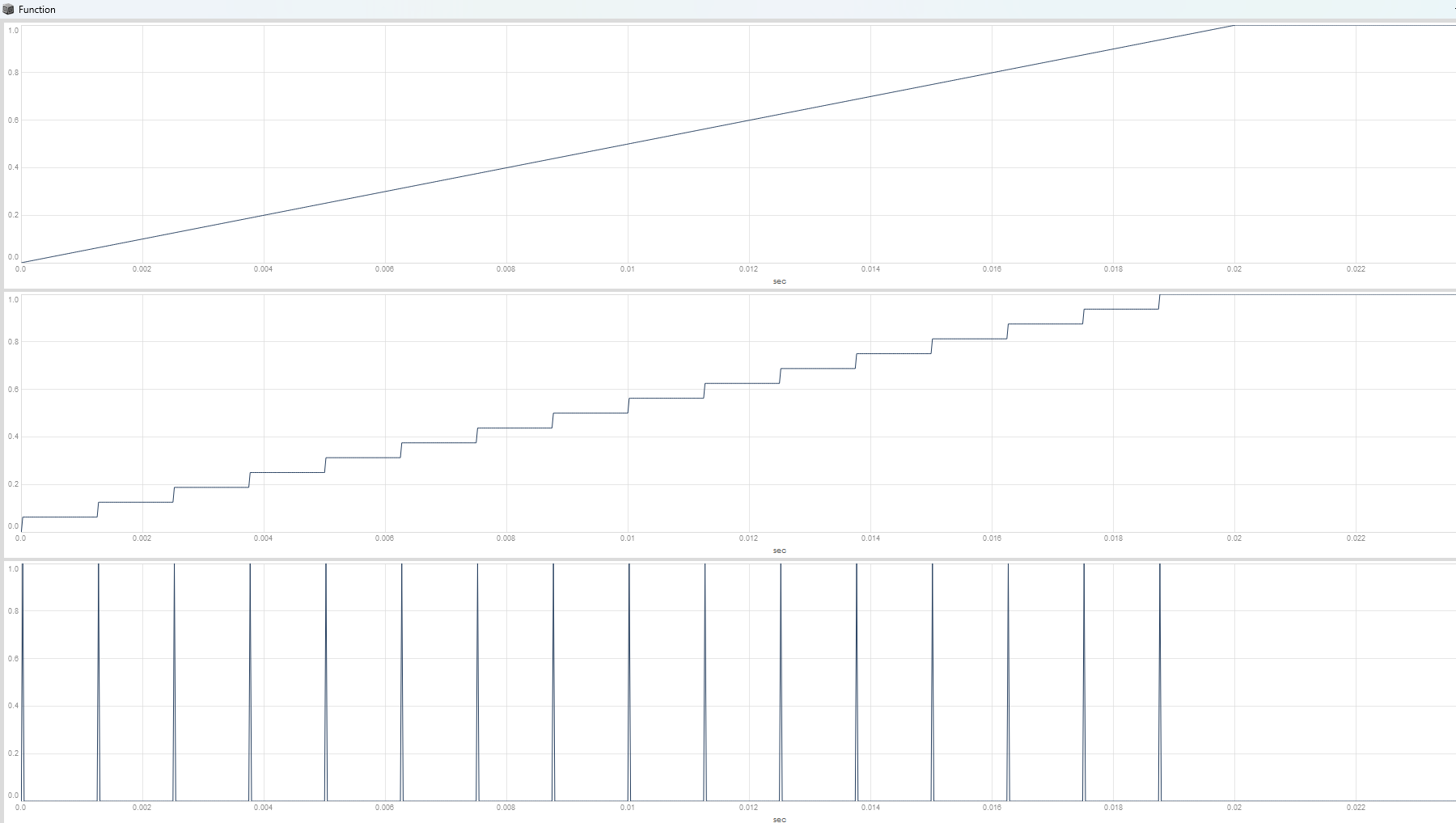
from your plot i have noticed, that you probably want to have a pulsaret train (several single carrier cycles) with a grain frequency trajectory.

In pulsar synthesis the grain duration is determined by the grain frequency, higher grain frequencies mean shorter grain durations and vice versa. In other types of microsound the grain duration is dependent on the trigger frequency instead. So for having this grain frequency trajectory per pulsaret train you cant use FM, because the grain durations would get shortened, if the grain frequency gets higher while beeing modulated.

Instead you could use Phase Modulation or Phase Distortion, which is when beeing implemented as “phase increment distortion” a subset of PM.

There are two types of phase distortion, the first is called “phase shaping”. Its similar to “wave shaping” where you take a signal and put it through a non-linear transfer function, but applied to the phase of a signal.

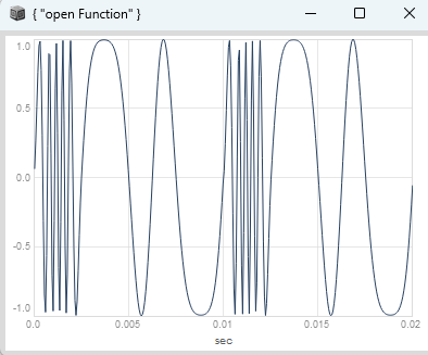
classic PD as “phase shaping”

(
var transferFunc = { |phase, skew|
	phase = phase.linlin(0, 1, skew.neg, 1 - skew);
	phase.bilin(0, skew.neg, 1 - skew, 0.5, 0, 1);
};

{
	var skew = \skew.kr(0.125);
	var phase = Phasor.ar(0, 100 * SampleDur.ir);
	cos(transferFunc.(phase, skew) * 2pi).neg;
}.plot(0.02);
)

With “phase increment distortion” you have a classic PM formula → phase + (mod * index), but add a non-linear unipolar modulation signal, like a window function (lets call this a frequency window even when beeing applied to the phase) to your linear phase.

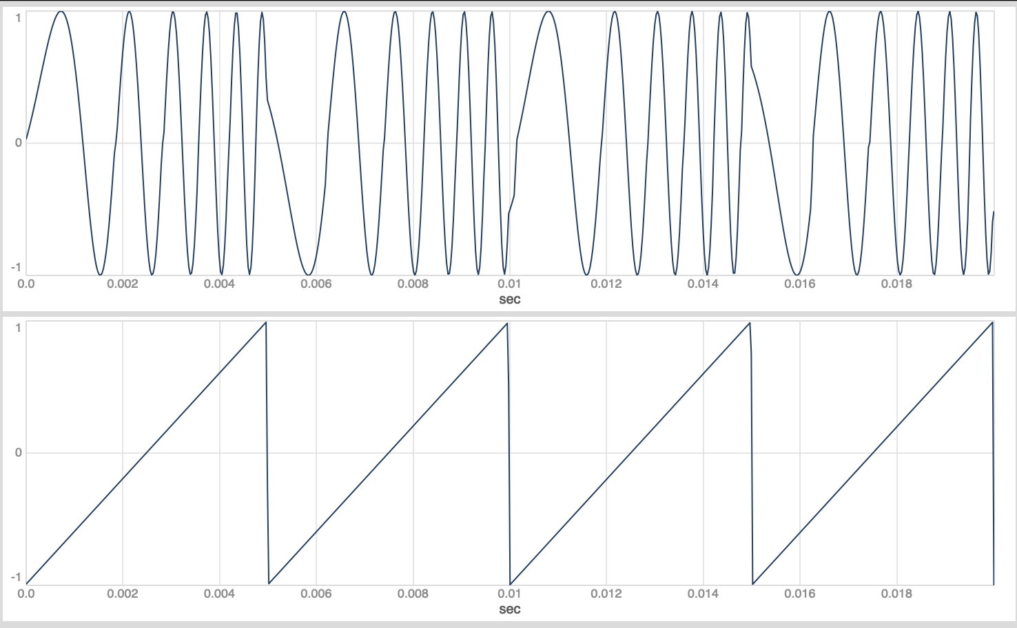
classic PD as “phase increment distortion”

(
var transferFunc = { |phase, skew|
	phase = phase.linlin(0, 1, skew.neg, 1 - skew);
	phase.bilin(0, skew.neg, 1 - skew, 1, 0, 0);
};

{
	var skew = \skew.kr(0.125);
	var phase = Phasor.ar(0, 100 * SampleDur.ir);
	cos(phase + (transferFunc.(phase, skew) * (0.5 - skew)) * 2pi).neg;
}.plot(0.02);
)

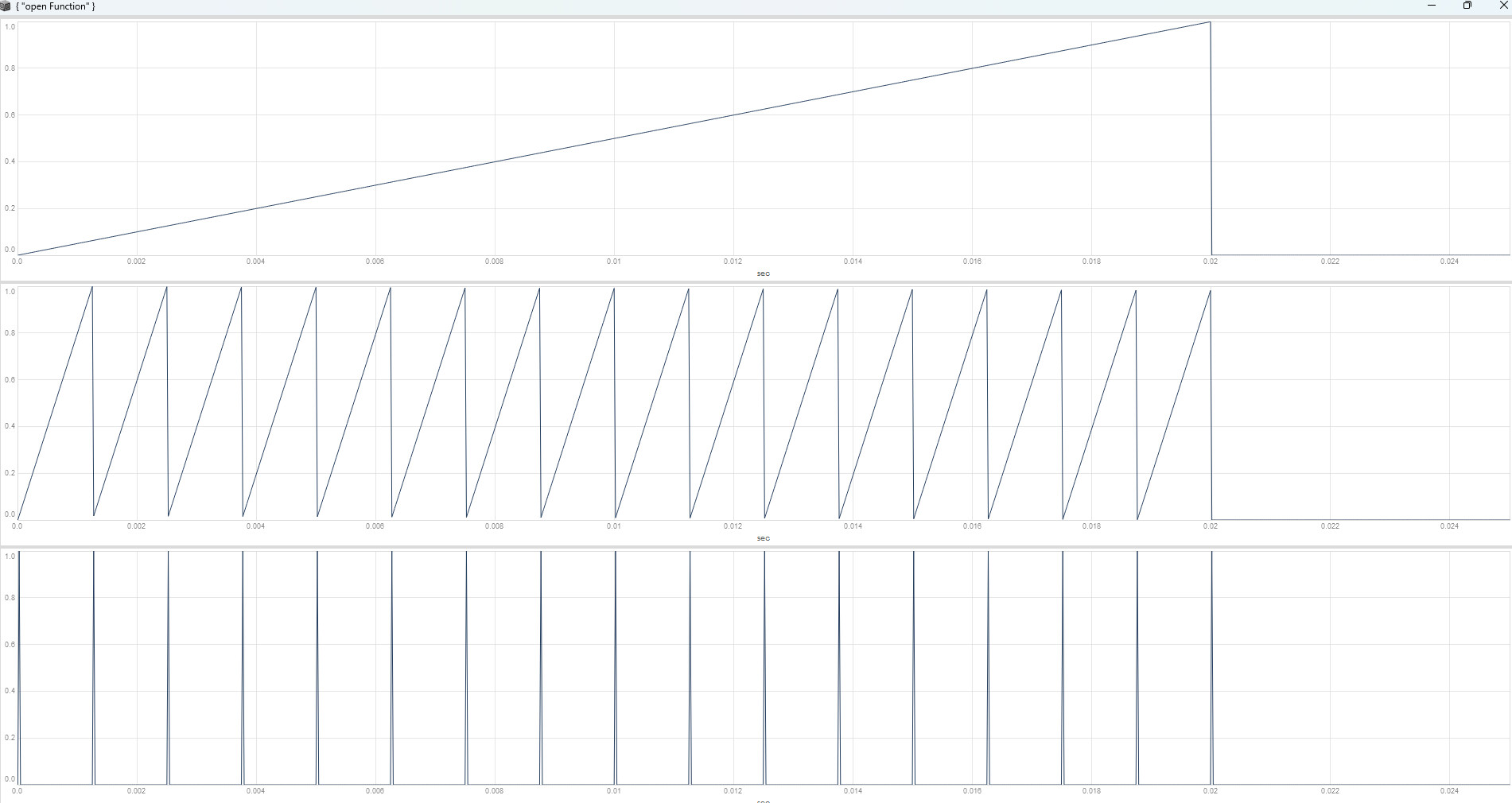
The beauty of the “phase increment distortion” method in our context is, that you dont have to use the same phase to drive your carrier and your modulator. This is perfect for pulsar synthesis. Because you want to use the grainPhase to drive your carrier and the windowPhase to drive the modulator.

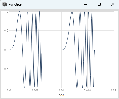
Here with a simple half sine cycle as a modulator. Use a different sign to change direction of the sweep and adjust the duty cycle with overlap to your liking. Also try out different modulation functions.

(
{
	var tFreq = 100;
	var trig = Impulse.ar(tFreq);
	var grainFreq = 800;
	var overlap = min(\overlap.kr(5), grainFreq / tFreq);

	var phase = Sweep.ar(trig, grainFreq);
	var windowPhase = phase / overlap;
	var rectWindow = windowPhase < 1;

	var mod = sin(windowPhase * pi);
	var sig = sin(phase + (mod * \index.kr(-1) * overlap / pi) * 2pi);

	sig * rectWindow;

}.plot(0.02);
)

grafik

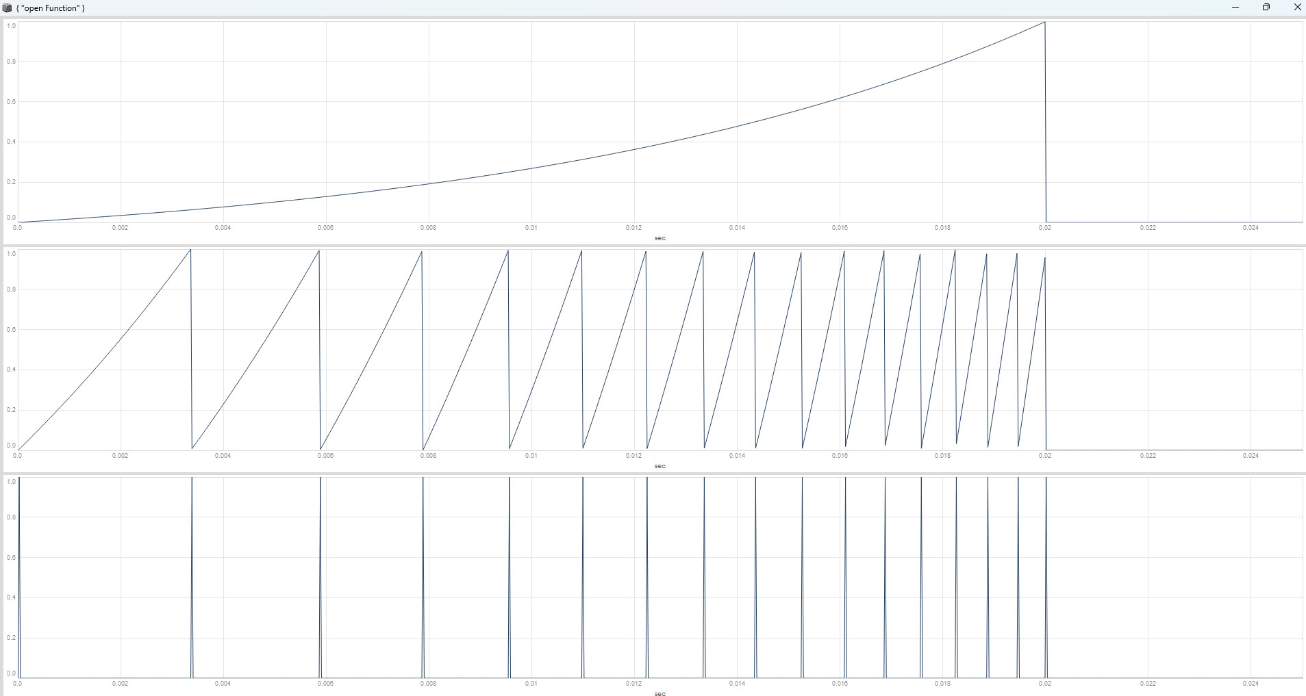
combine “phase shaping” and “phase increment distortion” for a more complex modulator, here the modulator has a skew param:

(
var transferFunc = { |phase, skew|
	phase = phase.linlin(0, 1, skew.neg, 1 - skew);
	phase.bilin(0, skew.neg, 1 - skew, 0.5, 0, 1);
};

{
	var tFreq = 100;
	var trig = Impulse.ar(tFreq);
	var grainFreq = 400;
	var overlap = min(\overlap.kr(4), grainFreq / tFreq);

	var phase = Sweep.ar(trig, grainFreq);
	var windowPhase = phase / overlap;
	var rectWindow = windowPhase < 1;

	var skew = \skew.kr(0.25);
	var mod = cos(transferFunc.(windowPhase, skew) * 2pi).neg * 0.5 + 0.5;
	var sig = sin(phase + (mod * (0.5 - skew) * \index.kr(4) * overlap) * 2pi);

	sig * rectWindow;
	
}.plot(0.02);
)

grafik

Thank you, this is spot on: I want a pulsaret train, and I want phase modulation or distortion :slight_smile:
Is there an advantage to using the sine or cosine function of the phase over using a buffered waveform and BufRd?

I think its better to have basic shapes and heavy modulation instead of complex static buffered shapes. But feel free to check out different buffered waveforms as carrier signals, window functions or modulators. The concept is the same.

Ah, good to know! I would have probably just used a buffered sine or cosine wave.

i just use sine waves with some additional harmonics as carriers. modulatable window functions for some params per pulsaret train with modulatable skew and width control and a modulation matrix with 4 modulators for each synthesis param (3 driven with subdivions of a main phasor and one chaotic one).

cool to add disperser, some saturation and filtering, but doing most of the post processing in ableton where i have better distortion plugins and can add EQ, multiband compression and convolution reverb more easily.

var disperser = { |in, fltFreq|
	var wet;
	wet = in;
	8.do {
		wet = Allpass1.ar(wet, fltFreq);
	};
	wet;
};

var softSaturation = { | in, curve|
	var k = 2 * curve / (1 - curve);
	(1 + k) * in / (1 + (k * in.abs));
};

I was trying to include some basic waveshaping with tanh at some point, but it never sounded all that great to me. Looking forward to trying your approach!

beside the so called “frequency window” you can add additional phase modulation, driven by a “modPhase”, I use an additional OnePole low pass filter to smooth out the phase modulation and an “index Window”

modSlope = grainSlope * \pmRatio.kr(3);
pmIndex = indexWindow * \pmIndex.kr(0);

modPhase = (modSlope * accumulator).wrap(0, 1);
pmod = sin(modPhases * 2pi) * pmIndex;
pmod = OnePole.ar(pmod, exp(-2pi * modSlope));

grainPhase = (grainSlope * accumulator).wrap(0, 1);
grainPhase = grainPhase + (freqWindow * (0.5 - skew) * \glissIndex.kr(0) * overlap);
grainPhase = grainPhase + (pmods / 2pi);

grains = sin(grainPhase * 2pi);

Sorry, I am not sure I follow what you are doing here. Would you mind explaining how you’d incorporate this into the code you shared above? Does this replace the modulator in the “phase increment distortion” example?

Lets pick the very first example i have shared, where i use an accumulator Duty.ar(SampleDur.ir, 0, Dseries(0, 1)); and mulitply it by different slopes to accumulate different phases for different signals, like a grainPhase which drives your carrier and a windowPhase which drives your grainWindow and accumulate yet another phase, a modPhase to drive our phase modulator.

(
var rampToSlope = { |phase|
	var history = Delay1.ar(phase);
	var delta = (phase - history);
	delta.wrap(-0.5, 0.5);
};

var rampToTrig = { |phase|
	var history = Delay1.ar(phase);
	var delta = (phase - history);
	var sum = (phase + history);
	var trig = (delta / sum).abs > 0.5;
	Trig1.ar(trig, SampleDur.ir);
};

var getSubSampleOffset = { |phase, trig|
	var slope = rampToSlope.(phase);
	var sampleCount = phase - (slope < 0) / slope;
	Latch.ar(sampleCount, trig);
};

var accumulatorSubSample = { |trig, subSampleOffset|
	var accum = Duty.ar(SampleDur.ir, trig, Dseries(0, 1));
	accum + subSampleOffset;
};

{
	var flux, triggerRate, stepPhase, stepSlope, stepTrigger, subSampleOffsets, accumulator;
	var windowSlope, windowPhase, maxOverlap, overlap;
	var modSlope, modPhase, pmod;
	var grainFreq, grainSlope, grainPhase, grainWindow, sig;
	
	flux = LFDNoise3.ar(\fluxMF.kr(10));
	flux = 2 ** (flux * \fluxMD.kr(3));
	
	triggerRate = \triggerRate.kr(20) * flux;
	stepPhase = (Phasor.ar(0, triggerRate * SampleDur.ir) - SampleDur.ir).wrap(0, 1);
	stepTrigger = rampToTrig.(stepPhase);
	stepSlope = rampToSlope.(stepPhase);

	subSampleOffsets = getSubSampleOffset.(stepPhase, stepTrigger);
	accumulator = accumulatorSubSample.(stepTrigger, subSampleOffsets);

	grainFreq = \grainFreq.kr(440) * flux;
	grainSlope = grainFreq * SampleDur.ir;
	grainPhase = (grainSlope * accumulator).wrap(0, 1);

	maxOverlap = grainSlope / Latch.ar(stepSlope, stepTrigger);
	overlap = min(\overlap.kr(30), maxOverlap);
	windowSlope = grainSlope / max(0.001, overlap);
	windowPhase = (windowSlope * accumulator).clip(0, 1);
	
	modSlope = grainSlope * \pmRatio.kr(3);
	modPhase = (modSlope * accumulator).wrap(0, 1);
	
	grainWindow = IEnvGen.ar(Env([0, 1, 0], [0.03, 0.97], [4.0, -4.0]), windowPhase);
	
	pmod = sin(modPhase * 2pi) * \pmIndex.kr(2);
	pmod = OnePole.ar(pmod, exp(-2pi * modSlope));
	
	sig = sin(grainPhase + (pmod / 2pi) * 2pi);

	sig = sig * grainWindow;

	sig!2 * 0.1;
	
}.play;
)

You can now adjust the pmRatio and the pmIndex.

2 Likes

Many thanks! I really appreciate you sharing this so generously. This is exactly what I was hoping to achieve.

1 Like

couldnt resist to add the additional flux modulator haha

Hahah, I would have almost missed that. Sounds fantastic!

haha thanks, yeah swap some waveforms, windows add some more modulation, masking,
spatialization, add multichannel expansion for overlapping grains etc. If you have any questions, feel free to ask :slight_smile:

2 Likes

Wow! Yeah, I am sure I’ll have some more questions, but this gives me enough to work through for now.

1 Like

OK, I do have a question, @dietcv. Going back to my original post and the first two pieces of code you posted where you demonstrate the use of an accumulator and how to subdivide a main phasor for slower LFOs: How do you modulate the trigger frequency here with an LFO driven by the same phasor as the grains?

hey,

The main phasor lets call it the “grain scheduler” is running at a certain frequency. This phasor could be subdivided or you can use it to accumulate new ramps at different rates to drive different windows or LFOs to modulate different params of your SynthDef. If you want to use the main phasor to modulate itself, you would need a feedback loop.

I think the best way of going about this is to have a “modulation phasor” and subdivide it to drive different LFOs to modulate different params and your “grain scheduler” which you use to accumulate different ramps at different rates to drive different window functions. The modulation phasor could also modulate the “trigger frequency” of your “grain scheduler”.

A different approach could be to trigger the single samples impulses from the language.
Instead of modulating the “trigger frequency” of your “grain scheduler” with an LFO, you could use a one-shot trigger from the language and get a fixed amount of single samples impulses per measure:

(
var rampToTrig = { |phase|
	var history = Delay1.ar(phase);
	var delta = (phase - history);
	var sum = (phase + history);
	var trig = (delta / sum).abs > 0.5;
	Trig1.ar(trig, SampleDur.ir);
};

{

	var trig, measurePhase, stepPhase, stepTrigger;

	trig = Impulse.ar(0);

	measurePhase = EnvGen.ar(Env(#[0, 0, 1], [0, \duration.kr(1 / 50)], \lin), trig).wrap(0, 1);
	measurePhase = measurePhase.lincurve(0, 1, 0, 1, \curve.kr(0));

	stepPhase = (measurePhase * \stepPerMeasure.kr(16)).wrap(0, 1);
	stepTrigger = rampToTrig.(stepPhase);

	[measurePhase, stepPhase, stepTrigger];
}.plot(0.025);
)

Additionally you could curve the measurePhase and get a fixed amount of exponentially spaced single sample triggers:

One thing to be aware of when doing this is:

The rampToTrig function does create a trigger when the step phase wraps from 1 to 0, so you dont get 16 triggers per measure in this case, but 17. To get 16 triggers per measure you cant wrap your main phasor. If you dont wrap it and instead of rampToTrig use .ceil and Changed, you get 16 single sample triggers. But in the microsound context you additionally need to calculate the slope of your grain scheduler to adjust your grain window per step, which would be not correct for the slope between the two last triggers, the slope is already a flat line after the second last trigger.

(
{

	var trig, measurePhase, stepTrigger, stepIndex;

	trig = Impulse.ar(0);

	measurePhase = EnvGen.ar(Env(#[0, 0, 1], [0, \duration.kr(1 / 50)], \lin), trig);
	measurePhase = measurePhase.lincurve(0, 1, 0, 1, \curve.kr(0));

	stepIndex = (measurePhase * \stepPerMeasure.kr(16)).ceil;
	stepTrigger = Changed.ar(stepIndex);

	[measurePhase, stepIndex / 16, stepTrigger];
}.plot(0.025);
)